🧠 阿头学 · 💬 讨论题

KV 缓存是大模型推理提速的基础，但这篇解释对真实瓶颈说得还不够狠

这篇文章对 KV 缓存“为什么能让解码变快”讲清楚了，但对“为什么推理依然很贵、真正卡在哪里”讲得明显过于乐观和简化。
打开原文 ↗

2026-05-11 原文链接 ↗

阅读简报

双语对照

完整翻译

原文

讨论归档

核心观点

历史K/V具有时间不变性：自回归生成中，已产出token的Key和Value向量在后续步骤中不会变更，逐token重算确实导致O(n²)的算力浪费，这是KV缓存的数学基础。
Prefill-Decode两阶段架构：首个token延迟（TTFT）本质是为整段prompt执行一次全量前向传播以构建缓存，后续decode仅计算单token并读取缓存，两者在计算特性上完全不同。
显存容量是并发瓶颈：以Qwen 2.5 72B为例，单请求的KV缓存可达数GB，在数百并发场景下总显存占用必然超过模型权重，因此上下文长度与并发用户数存在硬性的零和关系。
优化技术形成衍生链：为缓解显存灾难，GQA和MQA通过共享KV头压缩缓存，PagedAttention通过虚拟内存机制管理显存碎片，这些现代大模型标配技术都是KV缓存约束下的直接产物。
空间换时间存在物理天花板：KV缓存并非银弹，它只消除了K/V投影的重复计算，但Attention本身仍需对全缓存执行计算，且未解决显存带宽瓶颈，因此超长上下文的推理成本仍会随着序列长度线性上升。

跟我们的关联

对ATou：在构建Agent或长文本应用时，必须放弃"上下文越长越好"的线性思维，因为每轮对话的历史KV缓存会持续膨胀，直接推高单用户显存成本；下一步应优先采用Prompt Caching固化高频System Prompt，并对历史对话做摘要或RAG外置，以降低Prefill阶段的TTFT和显存占用。
对Neta：KV缓存的"Prefill-Decode"逻辑可直接映射为组织知识管理——建立SOP和共享知识库是一次性支付Prefill成本，后续项目执行只需增量解码（Decode），能避免团队陷入O(n²)的重复沟通；下一步应把高消耗、高重复的认知工作提前固化为可复用的"组织KV缓存"。
对Uota：评估AI应用出海或模型托管方案时，必须将"最大上下文长度"与"并发用户数"视为互斥变量而非独立卖点；下一步在核算Unit Economics时，需按目标并发量反推可承受的最大KV缓存总容量，并验证服务商是否部署了GQA/MQA和PagedAttention，否则超长上下文承诺只是不可持续的技术PR。

讨论引子

如果KV缓存的显存瓶颈是Transformer架构的内生性缺陷，那么Mamba、RWKV等无KV缓存的替代架构是否能在未来2-3年内突破现有推理成本曲线，取代Transformer在端侧部署的地位？
在Agent多轮工具调用场景中，历史观测的KV缓存会随轮

你每次使用 ChatGPT 或 Claude 时一定都注意到过，第一枚 token 明显要更久才会出现。接下来其余内容却几乎会立刻流式输出。

这背后其实是一个刻意为之的工程设计，叫作 KV 缓存，它的目的就是让大语言模型的推理更快。

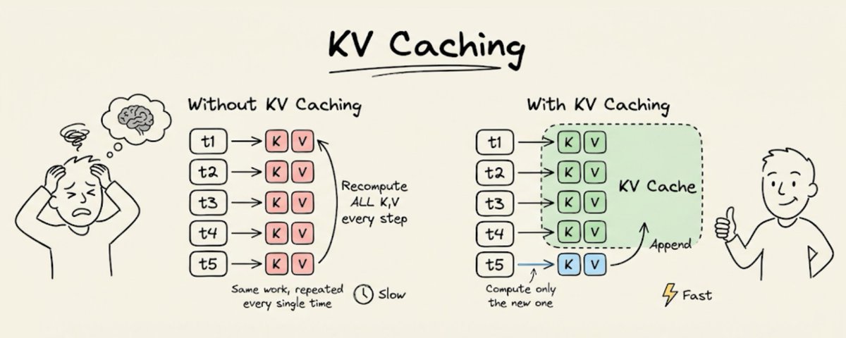
在进入技术细节之前，先看一组并排对比，看看使用 KV 缓存和不使用 KV 缓存时，大模型推理有什么差别。

现在我们从最基本的原理出发，来理解它是怎么工作的。

第 1 部分：大模型如何生成 token

Transformer 会处理所有输入 token，并为每个 token 产出一个隐藏状态。这些隐藏状态随后会被投影到词表空间，生成 logits，也就是词表中每个词对应的一个分数。

但真正重要的，只有最后一个 token 对应的 logits。你从中采样，得到下一个 token，把它追加到输入里，然后重复这个过程。

这里的关键洞见是，想生成下一个 token，你其实只需要最新那个 token 的隐藏状态。其余所有隐藏状态，都只是中间产物。

第 2 部分：Attention 实际上在计算什么

在 Transformer 的每一层里，每个 token 都会得到三个向量，分别是 query，也就是 Q，key，也就是 K，以及 value，也就是 V。Attention 会把 query 和 key 相乘得到分数，再用这些分数对 value 加权。

现在只看最后一个 token。

QK^T 的最后一行会用到：

最后一个 token 的 query 向量
序列中所有 token 的 key 向量

而这一行最终的 attention 输出会用到：

同一个 query 向量
所有的 key 和 value 向量

所以，为了计算我们唯一真正需要的那个隐藏状态，每一层 attention 都需要最新 token 的 Q，以及所有 token 的 K 和 V。

第 3 部分：这里面的重复计算

生成第 50 个 token 时，需要第 1 到第 50 个 token 的 K 和 V 向量。生成第 51 个 token 时，需要第 1 到第 51 个 token 的 K 和 V 向量。

而第 1 到第 49 个 token 的 K 和 V 向量，其实早就算过了。它们没有变化。输入相同，输出也相同。可模型还是会在每一步里把它们从头重算一遍。

这意味着每一步都会有 O(n) 的重复工作。放到整个生成过程中，就会浪费 O(n²) 的算力。

第 4 部分：怎么解决

办法就是，不要在每一步都重算所有 K 和 V 向量，而是把它们存起来。对于每个新 token：

只为最新的那个 token 计算 Q、K 和 V。
把新的 K 和 V 追加到缓存里。
从缓存中取出之前所有的 K 和 V 向量。
用新的 Q 对完整缓存中的 K 和 V 运行 attention。

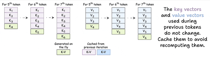
这就是 KV 缓存。每一层、每一步，只新增一个 K 和一个 V。其余全部直接从内存里取。

Attention 本身的计算量依然会随着序列长度增长，因为你还是要对所有 key 和 value 做 attention。但生成 K 和 V 的那些高开销投影，每个 token 只需计算一次，而不是每一步都算一次。

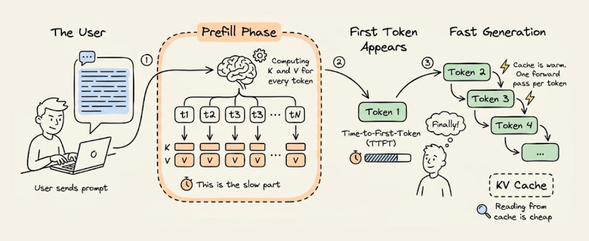
第 5 部分：首个 token 时间

现在你就能明白，为什么第一个 token 会慢了。

当你发出一个 prompt 时，模型会用一次完整的前向传播处理整段输入，计算并缓存每个 token 的 K 和 V 向量。这个过程叫 prefill 阶段，也是整个请求里计算最密集的部分。

一旦缓存预热完成，后续每个 token 都只需要做一次只含单个 token 的前向传播。

这段最初的延迟，就叫 time-to-first-token，简称 TTFT。prompt 越长，prefill 越久，等待时间也越长。优化 TTFT 本身又是一个很深的话题，比如 chunked prefill、speculative decoding、prompt caching，但底层逻辑始终一样：构建缓存很贵，读取缓存很便宜。

第 6 部分：取舍

KV 缓存是用内存换算力。每一层都要为每个 token 存储 K 和 V 向量。以 Qwen 2.5 72B 为例，80 层、32K 上下文、隐藏维度 8192，单个请求的 KV 缓存就可能占用数 GB 的 GPU 显存。当并发请求达到数百个时，它占用的显存往往会超过模型权重本身。

这也是为什么会有 grouped-query attention，也就是 GQA，以及 multi-query attention，也就是 MQA：让多个 query head 共享 key/value head，从而降低内存占用，同时质量损失很小。

这也是为什么把上下文长度翻倍会很难。窗口翻倍，每个请求的 KV 缓存也翻倍，并发用户数就会减少。

还有另一个思路叫 Paged attention，可以解决这个问题。我前不久在这里讲过：

总结

KV 缓存消除了自回归生成过程中的重复计算。之前的 token 总是会生成相同的 K 和 V 向量，所以只需要计算一次并存起来。每个新 token 只需要计算它自己的 Q、K 和 V。之后，attention 再对完整缓存执行计算。

实际中常常能带来 5 倍加速。代价是 GPU 显存，而在大规模场景下，这往往会成为真正的瓶颈。所有的大模型服务栈，比如 vLLM、TGI、TensorRT-LLM，都是建立在这个思路之上的。

到这里就讲完了。

如果你喜欢这篇教程：

可以在这里找到我 → @_avichawla

我每天都会分享关于 DS、ML、LLMs 和 RAGs 的教程与见解。

You must have seen it every time you use ChatGPT or Claude that the first token takes noticeably longer to appear. Then the rest stream out almost instantly.

你每次使用 ChatGPT 或 Claude 时一定都注意到过，第一枚 token 明显要更久才会出现。接下来其余内容却几乎会立刻流式输出。

Behind the scenes, it's a deliberate engineering decision called KV caching, and the purpose is to make LLM inference faster.

这背后其实是一个刻意为之的工程设计，叫作 KV 缓存，它的目的就是让大语言模型的推理更快。

Before we get into the technical details, here's a side-by-side comparison of LLM inference with and without KV caching:

在进入技术细节之前，先看一组并排对比，看看使用 KV 缓存和不使用 KV 缓存时，大模型推理有什么差别。

Now let's understand how it works, from first principles.

现在我们从最基本的原理出发，来理解它是怎么工作的。

Part 1: How LLMs generate tokens

第 1 部分：大模型如何生成 token

The transformer processes all input tokens and produces a hidden state for each one. Those hidden states get projected into vocabulary space, producing logits (one score per word in the vocabulary).

But only the logits from the last token matter. You sample from them, get the next token, append it to the input, and repeat.

但真正重要的，只有最后一个 token 对应的 logits。你从中采样，得到下一个 token，把它追加到输入里，然后重复这个过程。

This is the key insight: to generate the next token, you only need the hidden state of the most recent token. Every other hidden state is an intermediate byproduct.

这里的关键洞见是，想生成下一个 token，你其实只需要最新那个 token 的隐藏状态。其余所有隐藏状态，都只是中间产物。

Part 2: What Attention actually computes

第 2 部分：Attention 实际上在计算什么

Inside each transformer layer, every token gets three vectors: a query (Q), a key (K), and a value (V). Attention multiplies queries against keys for scores, then uses those scores to weight the values.

Now focus on just the last token.

现在只看最后一个 token。

The last row of QK^T uses:

QK^T 的最后一行会用到：

The query vector of the last token

最后一个 token 的 query 向量

All key vectors in the sequence

序列中所有 token 的 key 向量

The final attention output for that row uses:

而这一行最终的 attention 输出会用到：

The same query vector

同一个 query 向量

All key and value vectors

所有的 key 和 value 向量

So to compute the only hidden state we need, every attention layer requires Q from the latest token, and K and V from everything.

所以，为了计算我们唯一真正需要的那个隐藏状态，每一层 attention 都需要最新 token 的 Q，以及所有 token 的 K 和 V。

Part 3: The redundancy involved

第 3 部分：这里面的重复计算

Generating token 50 requires K and V vectors for tokens 1 through 50. Generating token 51 requires K and V vectors for tokens 1 through 51.

生成第 50 个 token 时，需要第 1 到第 50 个 token 的 K 和 V 向量。生成第 51 个 token 时，需要第 1 到第 51 个 token 的 K 和 V 向量。

The K and V vectors for tokens 1 through 49 were already computed. They haven't changed. Same inputs, same outputs. Yet the model recomputes them from scratch every step.

而第 1 到第 49 个 token 的 K 和 V 向量，其实早就算过了。它们没有变化。输入相同，输出也相同。可模型还是会在每一步里把它们从头重算一遍。

That's O(n) redundant work per step. Over an entire generation, O(n²) wasted compute.

这意味着每一步都会有 O(n) 的重复工作。放到整个生成过程中，就会浪费 O(n²) 的算力。

Part 4: The fix

第 4 部分：怎么解决

Instead of recomputing all K and V vectors at every step, store them. For each new token:

办法就是，不要在每一步都重算所有 K 和 V 向量，而是把它们存起来。对于每个新 token：

Compute Q, K, and V for only the newest token.

只为最新的那个 token 计算 Q、K 和 V。

Append the new K and V to the cache.

把新的 K 和 V 追加到缓存里。

Retrieve all previous K and V vectors from the cache.

从缓存中取出之前所有的 K 和 V 向量。

Run attention using the new Q against the full cached K and V.

用新的 Q 对完整缓存中的 K 和 V 运行 attention。

That's KV caching. One new K and one new V per layer per step. Everything else comes from memory.

这就是 KV 缓存。每一层、每一步，只新增一个 K 和一个 V。其余全部直接从内存里取。

The attention computation still scales with sequence length (you're attending over all keys and values). But the expensive projections to produce K and V happen only once per token, not once per step.

Part 5: Time-to-First-Token

第 5 部分：首个 token 时间

Now you can see why the first token is slow.

现在你就能明白，为什么第一个 token 会慢了。

When you send a prompt, the model processes the entire input in one forward pass, computing and caching K and V vectors for every token. This is the prefill phase, and it's the most compute-intensive part of the request.

Once the cache is warm, each subsequent token needs only a single forward pass with one token.

一旦缓存预热完成，后续每个 token 都只需要做一次只含单个 token 的前向传播。

That initial delay is called time-to-first-token (TTFT). Longer prompts mean longer prefills, which mean longer waits. Optimizing TTFT (chunked prefill, speculative decoding, prompt caching) is its own deep topic, but the dynamic is always the same: building the cache is expensive, reading from it is cheap.

Part 6: The Tradeoff

第 6 部分：取舍

KV caching trades compute for memory. Every layer stores K and V vectors for every token. For Qwen 2.5 72B (80 layers, 32K context, hidden dim 8192), the KV cache for a single request can consume several gigabytes of GPU memory. At hundreds of concurrent requests, it often exceeds the model weights themselves.

This is why grouped-query attention (GQA) and multi-query attention (MQA) exist: share key/value heads across query heads, cut memory, and minimal quality loss.

It's also why doubling context length is hard. Double the window, double the KV cache per request, fewer concurrent users.

这也是为什么把上下文长度翻倍会很难。窗口翻倍，每个请求的 KV 缓存也翻倍，并发用户数就会减少。

There is another idea called Paged attention, which solves this, and I talked about it here recently:

还有另一个思路叫 Paged attention，可以解决这个问题。我前不久在这里讲过：

tl;dr

总结

KV caching eliminates redundant computation during autoregressive generation. Previous tokens always produce the same K and V vectors, so you compute them once and store them. Each new token only needs its own Q, K, and V. Then, attention runs against the full cache.

5x speedup in practice. The cost is GPU memory, which becomes the binding constraint at scale. Every LLM serving stack (vLLM, TGI, TensorRT-LLM) builds on this idea.

That's a wrap!

到这里就讲完了。

If you enjoyed this tutorial:

如果你喜欢这篇教程：

Find me → @_avichawla

可以在这里找到我 → @_avichawla

Every day, I share tutorials and insights on DS, ML, LLMs, and RAGs.

我每天都会分享关于 DS、ML、LLMs 和 RAGs 的教程与见解。

You must have seen it every time you use ChatGPT or Claude that the first token takes noticeably longer to appear. Then the rest stream out almost instantly.

Behind the scenes, it's a deliberate engineering decision called KV caching, and the purpose is to make LLM inference faster.

Before we get into the technical details, here's a side-by-side comparison of LLM inference with and without KV caching:

Now let's understand how it works, from first principles.

Part 1: How LLMs generate tokens

The transformer processes all input tokens and produces a hidden state for each one. Those hidden states get projected into vocabulary space, producing logits (one score per word in the vocabulary).

But only the logits from the last token matter. You sample from them, get the next token, append it to the input, and repeat.

This is the key insight: to generate the next token, you only need the hidden state of the most recent token. Every other hidden state is an intermediate byproduct.

Part 2: What Attention actually computes

Now focus on just the last token.

The last row of QK^T uses:

The query vector of the last token
All key vectors in the sequence

The final attention output for that row uses:

The same query vector
All key and value vectors

So to compute the only hidden state we need, every attention layer requires Q from the latest token, and K and V from everything.

Part 3: The redundancy involved

Generating token 50 requires K and V vectors for tokens 1 through 50. Generating token 51 requires K and V vectors for tokens 1 through 51.

The K and V vectors for tokens 1 through 49 were already computed. They haven't changed. Same inputs, same outputs. Yet the model recomputes them from scratch every step.

That's O(n) redundant work per step. Over an entire generation, O(n²) wasted compute.

Part 4: The fix

Instead of recomputing all K and V vectors at every step, store them. For each new token:

Compute Q, K, and V for only the newest token.
Append the new K and V to the cache.
Retrieve all previous K and V vectors from the cache.
Run attention using the new Q against the full cached K and V.

That's KV caching. One new K and one new V per layer per step. Everything else comes from memory.

Part 5: Time-to-First-Token

Now you can see why the first token is slow.

Once the cache is warm, each subsequent token needs only a single forward pass with one token.

Part 6: The Tradeoff

This is why grouped-query attention (GQA) and multi-query attention (MQA) exist: share key/value heads across query heads, cut memory, and minimal quality loss.

It's also why doubling context length is hard. Double the window, double the KV cache per request, fewer concurrent users.

There is another idea called Paged attention, which solves this, and I talked about it here recently:

tl;dr

5x speedup in practice. The cost is GPU memory, which becomes the binding constraint at scale. Every LLM serving stack (vLLM, TGI, TensorRT-LLM) builds on this idea.

That's a wrap!

If you enjoyed this tutorial:

Find me → @_avichawla

Every day, I share tutorials and insights on DS, ML, LLMs, and RAGs.

📋 讨论归档

讨论进行中…