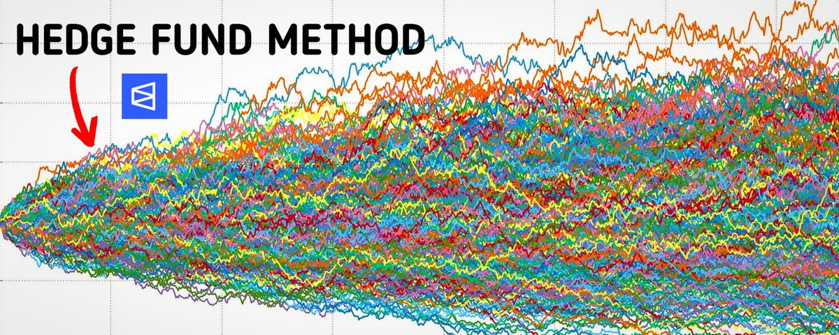
I'm going to break down exactly how hedge funds use prediction market data to build trading strategies and extract alpha that retail misses. I'll also share dataset of 400m+ trades going back to 2020.
Let's get straight to it.
Bookmark This -
I’m Roan, a backend developer working on system design, HFT-style execution, and quantitative trading systems. My work focuses on how prediction markets actually behave under load. For any suggestions, thoughtful collaborations, partnerships DMs are open.
The Dataset That Just Went Public
@beckerrjon released the largest publicly available prediction market dataset: 400 million+ trades from Polymarket and Kalshi going back to 2020. Complete market metadata, granular trade data, resolution outcomes, stored as Parquet files.
This is tick level data. Every trade has timestamp, price, volume, taker direction. The same granularity institutional data vendors charge $100K+ annually for in traditional markets.
**Now it's open source. This is massive. **
Before I break down what hedge funds are doing with this data, let me show you how to actually get it set up. Because unlike most articles that just talk theory, I'm giving you the exact steps to access institutional grade data yourself.
**How to Set Up the Dataset (Step by Step)
Prerequisites:**
Step 1: Install uv (Dependency Manager)
uv sync
Step 2: Clone the Repository
Step 3: Install Dependencies
This installs DuckDB, Pandas, Matplotlib and other analysis tools.
Step 4: Download the Dataset
This downloads data.tar.zst (36GB compressed) from Cloudflare R2 and extracts it to the data/ directory.
Extraction takes 5 to 30 minutes depending on your system (for me it took more than expected)
Step 5: Verify the Data
make setup
You should see hundreds of Parquet files containing trade data.
Congrats. You now have the same dataset hedge funds are analyzing.
The data is organized like this:
Each trade file is a Parquet file. What is Parquet file?
Parquet is a columnar storage format that lets you query billions of rows without loading everything into memory.
Now that you have it set up, let me show you what institutions are actually doing with this data.
ls data/polymarket/trades/
ls data/kalshi/trades/
How Hedge Funds Actually Use This Data
You think prediction markets are for betting on outcomes.
You're wrong.
Hedge funds use prediction market data as a laboratory for three things: empirical risk calibration, systematic bias detection and order flow analysis. The prediction market isn't where they deploy capital. It's where they extract patterns that inform billions in traditional market positions.
Here's exactly what they're doing with 400 million trades.
Method 1: Empirical Kelly Criterion with Monte Carlo Uncertainty Quantification
The Kelly Criterion is the foundation of quantitative position sizing.
Every institutional trader knows the formula:
f* = (p × b - q) / b
Where f* is the optimal fraction of capital to deploy, p is win probability, q is loss probability, and b represents the odds.
The problem with textbook Kelly: it assumes you know your edge with certainty.
Reality breaks this assumption immediately.
When your model estimates 6% edge on a trade, that's not ground truth. It's a point estimate with uncertainty. The true edge might be 3%. It might be 9%. You have a distribution, not a number.
Standard Kelly treats that 6% as fact. This is mathematically incorrect and leads to systematic overbetting.
Empirical Kelly solves this by incorporating uncertainty directly into the sizing calculation.
Here's how they implement it using the Becker dataset:
Phase 1: Historical Trade Extraction
Funds define their strategy criteria in precise terms.
For example: "Enter Yes when contract price is below $0.15 and our fundamental model estimates true probability above 0.25."
They filter the 400 million historical trades to find every instance where that exact pattern appeared. Not similar. Exact.
This gives them thousands of historical analogs. Each one has a known outcome because the dataset includes resolutions.
Phase 2: Return Distribution Construction
For each historical analog, they calculate what the realized return was. Win or loss. Magnitude. Timing.
This creates an empirical distribution of returns. Not a theoretical normal distribution. The actual, realized distribution of what happened when this pattern appeared in real markets.
Critical insight: this distribution is almost never normal. It has fat tails. It has skewness. It has kurtosis that would make a statistics professor wince.
Traditional models assume away these features. Empirical methods measure them directly.
Phase 3: Monte Carlo Resampling
Here's where it gets interesting mathematically.
The historical sequence of returns is just one possible path.
If the same trades had occurred in a different order, the equity curve would look completely different.
Returns of [+8%, -4%, +6%, -3%, +7%] average to the same number as [-4%, -3%, +6%, +7%, +8%], but the drawdown profiles are dramatically different. The first sequence never drops below 0%. The second sequence hits -7% drawdown immediately.
This is path dependency. And it matters enormously for risk management.
Monte Carlo resampling generates 10,000 alternative paths by randomly reordering the same historical returns. Each path has identical statistical properties but different realized risk profiles.
Phase 4: Drawdown Distribution Analysis
For each of the 10,000 simulated paths, calculate the maximum drawdown. The worst peak to trough decline.
Now you have a distribution of possible max drawdowns, not a single number. You can see the 50th percentile (median case), the 95th percentile (bad luck), the 99th percentile (disaster scenario).
This is where institutional risk management diverges from retail.
You: "My backtest shows 12% max drawdown, I can handle that."
Institutional: "The median path shows 12% drawdown, but the 95th percentile shows 31% drawdown. We need to size for the 95th percentile, not the median."
Phase 5: Uncertainty Adjusted Position Sizing
The final step is calculating position size that keeps the 95th percentile drawdown under institutional risk limits.
The math becomes:
f_empirical = f_kelly × (1 - CV_edge)
Where CV_edge is the coefficient of variation (standard deviation / mean) of edge estimates across the Monte Carlo simulations.
High uncertainty → large CV → aggressive haircut to position size.
Low uncertainty → small CV → sizing closer to theoretical Kelly.
Consider an illustrative application of this methodology:
A quantitative strategy: Long contracts under $0.20 where model estimates true probability > 0.30
Using historical pattern matching on the Becker dataset and Monte Carlo resampling:
Standard Kelly calculation might suggest: 20%+ position sizing
After volatility adjustment: ~15-20% sizing
After Monte Carlo uncertainty adjustment (typical CV: 0.3-0.5): 10-15% sizing
Conservative deployment allowing for model risk: 8-12%
The difference between ignoring uncertainty (20%+ sizing) and incorporating it (10% sizing) is the difference between probable ruin and steady compounding over time.
Why This Matters:
Every retail trader using Kelly is using the textbook version.
They're overbetting systematically because they're not accounting for uncertainty in their edge estimates.
Institutions using empirical Kelly with Monte Carlo are sizing for the distribution of possible outcomes, not the point estimate.
Over time, this creates massive divergence. The retail trader experiences a 40% drawdown that wipes out years of gains. The institutional trader never exceeds 20% drawdown and compounds smoothly.
Same strategy. Different position sizing methodology. Completely different outcomes.
Method 2: Calibration Surface Analysis Across Price and Time Dimensions
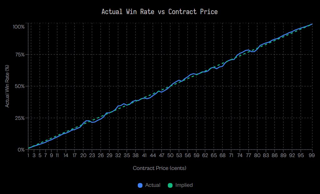
Standard calibration analysis plots implied probability versus realized frequency.
At price $0.30 (30% implied), how often did that outcome actually occur? If it occurred 30% of the time, the market was calibrated. If 25%, it was overpriced. If 35%, it was underpriced.
This is one dimensional analysis. Price only.
Institutions build calibration surfaces adding the time dimension: how does calibration change as resolution approaches?
The Framework:
Define C(p, t) as the calibration function where:
-
p represents contract price (0 to 100)
-
t represents time remaining until resolution (measured in days)
-
C(p, t) returns the empirical probability that outcome occurs
In perfectly calibrated markets, C(p, t) = p for all p and t.
In reality, C(p, t) varies systematically with both price and time.
What Jon Becker's Research Actually Shows:
Analysis of 72.1 million Kalshi trades reveals the longshot bias is real and measurable.
At extreme low probabilities (1-cent contracts):
At mid probabilities (50-cent contracts):
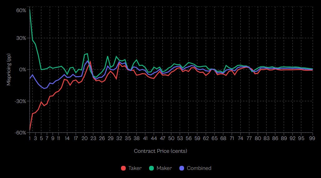
The research confirms takers exhibit negative excess returns at 80 of 99 price levels, proving systematic mispricing across the probability spectrum.
The Institutional Hypothesis on Time Dimension:
While Becker's published research focused on price based calibration, institutions extend this framework temporally based on behavioral finance theory.
The hypothesis: longshot bias should vary with time to resolution because the psychological drivers change.
Early Period (far from resolution): Retail sentiment dominates. Limited information exists. People buy lottery tickets based on hope rather than probability. This should maximize longshot bias.
Mid Period: Information accumulates. Sophisticated participants enter. Prices should converge toward fundamentals as the informational environment improves.
Late Period (near resolution): Information revelation accelerates. Outcomes that were always unlikely become obviously unlikely. The hypothesis suggests potential bias reversal as hope capitulates, but this requires empirical validation.
The Strategy Framework:
Time varying filter rules based on established behavioral patterns:
Far from resolution: The longshot bias documented by Becker is likely strongest here. Strategy: systematically fade low probability contracts where retail enthusiasm dominates.
Mid range: Peak efficiency period as information and liquidity improve. Strategy: reduce activity or focus on other edges.
Near resolution: Information asymmetry should collapse. Strategy: exploit any remaining mispricing but with awareness that efficiency typically improves.
Mathematical Formalization:
The mispricing function:
M(p, t) = C(p, t) - p/100
Where M represents systematic mispricing in percentage points.
Institutional entry rules would be:
Enter short when M(p, t) > threshold (overpriced)
Enter long when M(p, t) < -threshold (underpriced)
Stay flat when |M(p, t)| < threshold (fair)
The threshold is calibrated to transaction costs and required risk adjusted returns.
Why This Matters:
Becker's research proves the longshot bias exists at the price dimension. The documented -57% mispricing at 1-cent contracts is enormous and systematic.
Institutions hypothesize this bias varies with time, though empirical validation requires analysis of the full temporal dataset.
The framework is sound: behavioral biases driven by hope, fear, and information asymmetry should logically vary as resolution approaches.
Whether the specific pattern is early bias → mid efficiency → late reversal, or some other temporal structure, requires running the analysis on the 400 million trade dataset.
What we know for certain from verified research:
-
Longshot bias exists and is measurable (-57% at 1-cent)
-
It varies across the probability spectrum
-
Takers systematically lose at 80 of 99 price levels
-
The bias creates structural opportunity
What institutions test empirically:
-
How this bias changes with time to resolution
-
Whether patterns are stable across market categories
-
Optimal threshold levels for entry and exit
-
Transaction cost adjusted profitability
The calibration surface methodology provides the framework. The Becker dataset provides the laboratory. The empirical analysis determines which specific patterns exist and are tradeable.
# On Mac/Linux
curl -LsSf https://astral.sh/uv/install.sh | sh

# On Windows (PowerShell)
irm https://astral.sh/uv/install.ps1 | iex
Method 3: Order Flow Decomposition and Maker Versus Taker Profitability
This is the most subtle edge and the one retail traders never consider.
Every trade has two participants: a maker who provided liquidity and a taker who consumed it.
The maker posted a limit order. They waited.
The taker crossed the spread. They paid for immediacy.
Jon Becker's dataset tags every trade with the taker side. This means you can separate the population into makers and takers and analyze their profitability independently.
What Becker's Research Actually Reveals:
Analysis of 72.1 million Kalshi trades with resolution outcomes shows a stark asymmetry.
At 1-cent contracts (extreme longshots):
**At 50-cent contracts:
**
data/
├── polymarket/
│   ├── markets/               # Market metadata (titles, outcomes, status)
│   └── trades/                # Every trade (price, volume, timestamp)
└── kalshi/
    ├── markets/               # Same structure for Kalshi
    └── trades/
-
Taker mispricing: -2.65%
-
Maker mispricing: +2.66%
Aggregate findings:
-
Takers exhibit negative excess returns at 80 of 99 price levels
-
Makers buying YES: +0.77% excess return
-
Makers buying NO: +1.25% excess return
-
Statistical symmetry (Cohen's d ≈ 0.02) indicates makers don't predict better, they just structure better
This is not a small difference.
Takers, as a population, are systematically wrong. Not 50/50 coinflip wrong. Persistently, measurably wrong at 80% of all price levels.
Why Takers Lose:
Becker's research identifies the core insight: makers profit via structural arbitrage, not superior forecasting ability.
The near identical excess returns for makers buying YES (+0.77%) versus NO (+1.25%) proves they're not picking winners. They're exploiting a costly preference in the taker population.
Taker behavior reveals urgency. You cross the spread because you value execution certainty over price. This urgency correlates with behavioral bias.
First: Information asymmetry misperception. Takers believe they're acting on valuable information. Most aren't. They're reacting to public information emotionally, not privately.
Second: Affirmative bias. Becker's research shows takers exhibit "a costly preference for affirmative, longshot outcomes." They disproportionately buy YES on longshots, systematically overpaying.
Makers, conversely, demonstrate patience. By definition, they wait. This patience filters out emotional urgency.
Additionally, makers optimize for spread capture, not outcome prediction. Over time, spread collection plus the structural edge versus biased taker flow generates consistent positive expectation.
The Math:
Expected maker profit per filled order:
E[Profit_maker] = spread_capture + edge_vs_takers
Where:
From Becker's verified data:
-
Maker edge vs takers: +0.77% to +1.25% depending on position direction
-
This edge exists across 80 of 99 price levels
-
The edge is structural, not informational (proven by symmetric YES/NO performance)
If you provide liquidity consistently across many markets, you earn this edge repeatedly without needing superior forecasting ability.
But there's risk.
Inventory Risk: As a maker, you accumulate positions. You're long some markets, short others. If correlations shift or markets move against you, drawdowns occur before mean reversion.
Adverse Selection Risk: Not all takers are uninformed. As Becker notes, "sophisticated traders cross the spread to act on time sensitive information." Large orders may signal informed flow. You risk getting picked off.
Volume Evolution: Becker's research shows market maturity matters. In early low volume periods, even makers lost to relatively informed takers. The volume surge attracted professional liquidity providers who could then extract value at all price points.
The Institutional Market Making Framework:
Quote two sided markets with positive expected spread capture.
Allow small fills that represent retail taker flow (these have the documented bias).
Flag large fills for review (potential sophisticated participants).
Monitor aggregate inventory exposure and hedge when thresholds are exceeded.
Target consistent returns from structural edge, not outcome prediction.
Why This Matters:
Retail traders are almost always takers. They see a market, they click buy, they cross the spread.
By doing this, they're entering with a population that Becker's research proves has negative excess returns at 80% of all price levels.
At extreme longshots (1-cent contracts), takers underperform by 57%. Even at mid probabilities (50-cent), they underperform by 2.65%.
Institutions providing liquidity collect the other side of that edge.
Same markets. Different approach. Structural advantage proven by 72.1 million trades.
The Research Conclusion:
Becker's analysis demonstrates that wealth systematically transfers from liquidity takers to liquidity makers, driven by behavioral biases and market microstructure, not superior forecasting ability by makers.
The documented taker preference for affirmative, longshot outcomes creates the structural opportunity. The maker patience and spread capture methodology harvests it.
This is not theory. This is measured, verified reality from the largest prediction market dataset ever analyzed.
git clone https://github.com/Jon-Becker/prediction-market-analysis
cd prediction-market-analysis
The Institutional Edge is not Information
Here's what retail gets wrong about hedge funds.
They assume hedge funds win because they have better information. Better research. Better models. Better predictions.
That's not where the edge is.
The edge is in:
-
Risk management: Sizing positions for the distribution of outcomes, not the point estimate. Monte Carlo uncertainty adjustment prevents ruin.
-
Time-varying strategies: Exploiting calibration patterns that change as resolution approaches. Selling early bias. Buying late reversal.
-
Structural positioning: Being the maker instead of the taker. Collecting spread and adverse selection edge from impatient counterparties.
None of these require better prediction. They require better process.
The Becker dataset gives you the laboratory to build that process.
400 million trades. Every outcome known. Every pattern measurable.
Retail will use this data to backtest their predictions.
Institutions will use this data to calibrate their risk management, identify time-varying biases and measure structural edges.
***I have an idea for the most insane prediction market experiment ever built on this dataset - reply YES if you want me to do it
7K people already follow this journey, join them so you don't miss what's next.***


Link: http://x.com/i/article/2022988148943601665