这不是一份技巧清单。
这是一段故事——从一次抛硬币开始,最终抵达机构级的仿真引擎。
每一节都建立在前一节之上。你若跳读,数学就会断裂;按顺序读下去,读到最后,你将拿到从上到下每一层都可运行的代码。
免责声明: ***非金融建议,请自行研究
第一部分:那次让一切崩塌的抛硬币
你盯着 Polymarket 上的一份合约:“美联储会在 3 月降息吗?”YES 的成交价是 $0.62。
你的直觉说:这就是 62% 的概率。也许你觉得它应该是 70%。于是你买入。
恭喜你。你刚刚做了几乎每个散户交易者都会做的事:你把预测市场合约当成一枚带已知偏置的硬币,估出你自己的“偏置”,然后把差额押上去。
-
你不知道该对自己的 70% 估计有多自信。
-
你不知道明天就业报告出来后,它应该如何变化。
-
你不知道它与 Polymarket 上另外六个与美联储相关的合约是怎样相关的。
-
你不知道从现在到结算之间的价格路径,是否会让你即便最终判断正确也能在途中以盈利退出。
抛硬币只有一个参数:p。
而嵌入在一组相关事件的组合中、信息流随时间变化、带着订单簿动态与执行风险的预测市场合约,参数却有几十个。
第二部分:蒙特卡洛——那块没人足够尊重的基石
本文中的所有仿真,最终都可以归结为蒙特卡洛:从分布中抽样、计算统计量、重复。
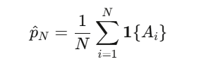
事件概率 p=P(A) 的估计量,就是样本均值:
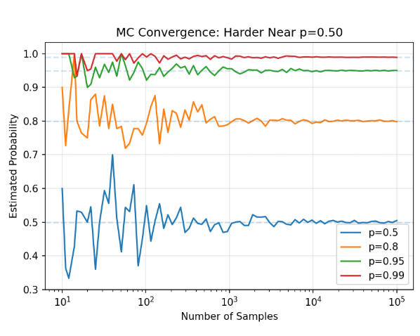
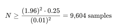
中心极限定理给出收敛速率:O(N^{-1/2}),且方差 Var(p^_N)=p(1−p)/N。
方差在 p=0.5 时达到最大。 平台上价格在 50 美分附近的合约,最不确定、交易也最活跃——也正是你的蒙特卡洛估计最不精确的地方。
当 p=0.50 时,要在 95% 置信度下达到 ±0.01 的精度:
这还算可控。但一旦你需要模拟的是路径而不只是终点,事情会迅速变糟。
你的第一个可运行仿真
目标: 估计一个与资产挂钩的二元合约兑现的概率(例如:“AAPL 会在 3 月 15 日收盘高于 $200 吗?”)
这能用。对单个合约、单个标的、并且假设对数正态动态时,它就能工作。真实的预测市场会把这些假设逐条打碎。
评估你的仿真
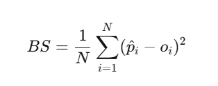
在改进仿真之前,我们需要一种衡量它有多好的办法。布里尔分数(Brier Score)是标准的校准指标:
import numpy as np
from scipy.special import expit, logit  # sigmoid and logit

class PredictionMarketParticleFilter:
    """
    Sequential Monte Carlo filter for real-time event probability estimation.

    Usage during a live event (e.g., election night):
        pf = PredictionMarketParticleFilter(prior_prob=0.50)
        pf.update(observed_price=0.55)   # market moves on early returns
        pf.update(observed_price=0.62)   # more data
        pf.update(observed_price=0.58)   # partial correction
        print(pf.estimate())             # filtered probability
    """
    def __init__(self, N_particles=5000, prior_prob=0.5,
                 process_vol=0.05, obs_noise=0.03):
        self.N = N_particles
        self.process_vol = process_vol
        self.obs_noise = obs_noise

        # Initialize particles around prior
        logit_prior = logit(prior_prob)
        self.logit_particles = logit_prior + np.random.normal(0, 0.5, N_particles)
        self.weights = np.ones(N_particles) / N_particles
        self.history = []

    def update(self, observed_price):
        """Incorporate a new observation (market price, poll result, etc.)"""
        # 1. Propagate: random walk in logit space
        noise = np.random.normal(0, self.process_vol, self.N)
        self.logit_particles += noise

        # 2. Convert to probability space
        prob_particles = expit(self.logit_particles)

        # 3. Reweight: likelihood of observation given each particle
        log_likelihood = -0.5 * ((observed_price - prob_particles) / self.obs_noise)**2
        log_weights = np.log(self.weights + 1e-300) + log_likelihood

        # Normalize in log space for stability
        log_weights -= log_weights.max()
        self.weights = np.exp(log_weights)
        self.weights /= self.weights.sum()

        # 4. Check ESS and resample if needed
        ess = 1.0 / np.sum(self.weights**2)
        if ess < self.N / 2:
            self._systematic_resample()

        self.history.append(self.estimate())

    def _systematic_resample(self):
        """Systematic resampling - lower variance than multinomial."""
        cumsum = np.cumsum(self.weights)
        u = (np.arange(self.N) + np.random.uniform()) / self.N
        indices = np.searchsorted(cumsum, u)
        self.logit_particles = self.logit_particles[indices]
        self.weights = np.ones(self.N) / self.N

    def estimate(self):
        """Weighted mean probability estimate."""
        probs = expit(self.logit_particles)
        return np.average(probs, weights=self.weights)

    def credible_interval(self, alpha=0.05):
        """Weighted quantile-based credible interval."""
        probs = expit(self.logit_particles)
        sorted_idx = np.argsort(probs)
        sorted_probs = probs[sorted_idx]
        sorted_weights = self.weights[sorted_idx]
        cumw = np.cumsum(sorted_weights)
        lower = sorted_probs[np.searchsorted(cumw, alpha/2)]
        upper = sorted_probs[np.searchsorted(cumw, 1 - alpha/2)]
        return lower, upper

# --- Simulate election night ---
pf = PredictionMarketParticleFilter(prior_prob=0.50, process_vol=0.03)

# Incoming observations (market prices as new data arrives)
observations = [0.50, 0.52, 0.55, 0.58, 0.61, 0.63, 0.60,
                0.65, 0.70, 0.75, 0.80, 0.85, 0.90, 0.95]

print("Election Night Tracker:")
print(f"{'Time':>6}  {'Observed':>10}  {'Filtered':>10}  {'95% CI':>20}")
print("-" * 52)

for t, obs in enumerate(observations):
    pf.update(obs)
    ci = pf.credible_interval()
    print(f"{t:>5}h  {obs:>10.3f}  {pf.estimate():>10.3f}  ({ci[0]:.3f}, {ci[1]:.3f})")
布里尔分数低于 0.20 就算不错。
低于 0.10 则非常优秀。
历史上最好的选举预测机构(538、Economist)在总统选举中的成绩大致在 0.06–0.12。
如果你的仿真能超过这个水平,你就有优势。
第三部分:当 100,000 次抽样仍然不够
现在,故事升级了。
Polymarket 上有许多极端事件合约。“标普 500 会在一周内下跌 20% 吗?”的价格是 $0.003。用朴素的蒙特卡洛跑 100,000 次抽样,你可能一次都碰不到,或者只碰到一次。
你的估计要么是 0.00000,要么是 0.00001——两者都毫无用处。
这不是一个理论问题。这正是多数散户无法正确评估尾部风险合约的原因。
让稀有事件变得常见
重要性采样(importance sampling)用一种会过度采样稀有区域的概率测度替换原测度,然后再用似然来修正偏差。
似然比(likelihood ratio)或 Radon–Nikodym 导数
它本身并不能直接拿来用,但它告诉你:你应该朝什么方向去逼近。
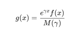
实践中真正的主力是指数倾斜(exponential tilting)。
如果你的标的服从一个随机游走,其增量 Δ_i 的矩母函数为 M(γ)=E[e^γΔ],你可以对分布进行倾斜:
选择 γ,让稀有事件变成“典型事件”。对那类在某个和超过巨大阈值时支付的合约,γ 满足 Lundberg 方程 M(γ)=1。
用于尾部风险合约的重要性采样
对极端合约而言,IS 可以把方差降低 100–10,000 倍。
这意味着:100 次 IS 抽样的精度,可能胜过 1,000,000 次朴素抽样。
这不是边际提升。这是“我们没法给它定价”和“我们在交易它”之间的差别。
第四部分:用于实时更新的序贯蒙特卡洛
但当故事从静态估计转向动态仿真时,你该怎么做?
想象一下: 那是选举之夜,东部时间晚上 8:01。佛罗里达刚刚关闭投票。早期计票显示,一方相对另一方出现了 3 个百分点的摆动。
你的模型需要立刻更新:把这个新数据点纳入概率估计,并且不仅是佛州,还包括俄亥俄、宾夕法尼亚、密歇根,以及所有相关的州。
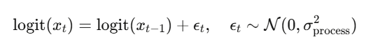
这就是滤波(filtering)问题,对应的工具是序贯蒙特卡洛(Sequential Monte Carlo)——粒子滤波。
状态空间模型
定义:
-
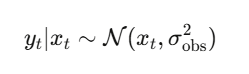
隐藏状态 x_t:事件的“真实”概率(不可观测)
-
观测 y_t:市场价格、民调结果、计票数、新闻信号
状态通过logit 随机游走演化(保证概率有界):
def brier_score(predictions, outcomes):
    """Evaluate simulation calibration."""
    return np.mean((np.array(predictions) - np.array(outcomes))**2)

# Compare two models
model_A_preds = [0.7, 0.3, 0.9, 0.1]  # sharp, confident
model_B_preds = [0.5, 0.5, 0.5, 0.5]  # always uncertain
actual_outcomes = [1, 0, 1, 0]

print(f"Model A Brier: {brier_score(model_A_preds, actual_outcomes):.4f}")  # 0.05
print(f"Model B Brier: {brier_score(model_B_preds, actual_outcomes):.4f}")  # 0.25
观测是对真实状态的带噪读数:
1. INITIALIZE: Draw x_0^{(i)} ~ Prior  for i = 1,...,N
   Set weights w_0^{(i)} = 1/N

2. FOR each new observation y_t:
   a. PROPAGATE:  x_t^{(i)} ~ f( · | x_{t-1}^{(i)} )
   b. REWEIGHT:   w_t^{(i)} ∝ g( y_t | x_t^{(i)} )
   c. NORMALIZE:  w̃_t^{(i)} = w_t^{(i)} / Σ_j w_t^{(j)}
   d. RESAMPLE if ESS = 1/Σ(w̃_t^{(i)})² < N/2
Bootstrap 粒子滤波
该算法维持 N 个“粒子”——每一个都是对真实概率的一种假设;随着数据到来,它们会被重新赋权:
用于实时预测市场的粒子滤波
为什么这比直接用市场价格更好?
因为粒子滤波会平滑噪声并传播不确定性。
当市场在一笔交易后从 $0.58 猛跳到 $0.65,滤波器会意识到真实概率未必真的变化这么大;它会根据观测过程本身的波动性,来“收敛”这次更新幅度。
第五部分:三种可叠加的方差缩减技巧
在离开蒙特卡洛疆域之前,这里有三种技巧——它们能与上述一切乘法式叠加。
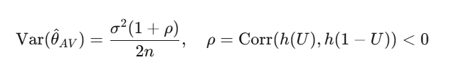
免费的对称性
当支付函数是单调的(而二元合约永远如此:价格越高意味着越可能超过执行价),方差缩减是有保证的:
import numpy as np
from scipy.stats import norm, t as t_dist

def simulate_correlated_outcomes_gaussian(probs, corr_matrix, N=100_000):
    """Gaussian copula no tail dependence."""
    d = len(probs)
    L = np.linalg.cholesky(corr_matrix)
    Z = np.random.standard_normal((N, d))
    X = Z @ L.T
    U = norm.cdf(X)
    outcomes = (U < np.array(probs)).astype(int)
    return outcomes

def simulate_correlated_outcomes_t(probs, corr_matrix, nu=4, N=100_000):
    """Student-t copula symmetric tail dependence."""
    d = len(probs)
    L = np.linalg.cholesky(corr_matrix)
    Z = np.random.standard_normal((N, d))
    X = Z @ L.T

    # Divide by sqrt(chi-squared / nu) to get t-distributed
    S = np.random.chisquare(nu, N) / nu
    T = X / np.sqrt(S[:, None])
    U = t_dist.cdf(T, nu)
    outcomes = (U < np.array(probs)).astype(int)
    return outcomes

def simulate_correlated_outcomes_clayton(probs, theta=2.0, N=100_000):
    """Clayton copula (bivariate) lower tail dependence."""
    # Marshall-Olkin algorithm
    V = np.random.gamma(1/theta, 1, N)
    E = np.random.exponential(1, (N, len(probs)))
    U = (1 + E / V[:, None])**(-1/theta)
    outcomes = (U < np.array(probs)).astype(int)
    return outcomes

# --- Compare tail behavior ---
probs = [0.52, 0.53, 0.51, 0.48, 0.50]  # 5 swing state probabilities
state_names = ['PA', 'MI', 'WI', 'GA', 'AZ']

corr = np.array([
    [1.0, 0.7, 0.7, 0.4, 0.3],
    [0.7, 1.0, 0.8, 0.3, 0.3],
    [0.7, 0.8, 1.0, 0.3, 0.3],
    [0.4, 0.3, 0.3, 1.0, 0.5],
    [0.3, 0.3, 0.3, 0.5, 1.0],
])

N = 500_000

gauss_outcomes = simulate_correlated_outcomes_gaussian(probs, corr, N)
t_outcomes = simulate_correlated_outcomes_t(probs, corr, nu=4, N=N)

# P(sweep all 5 states)
p_sweep_gauss = gauss_outcomes.all(axis=1).mean()
p_sweep_t = t_outcomes.all(axis=1).mean()

# P(lose all 5 states)
p_lose_gauss = (1 - gauss_outcomes).all(axis=1).mean()
p_lose_t = (1 - t_outcomes).all(axis=1).mean()

# If independent
p_sweep_indep = np.prod(probs)
p_lose_indep = np.prod([1-p for p in probs])

print("Joint Outcome Probabilities:")
print(f"{'':>25}  {'Independent':>12}  {'Gaussian':>12}  {'t-copula':>12}")
print(f"{'P(sweep all 5)':>25}  {p_sweep_indep:>12.4f}  {p_sweep_gauss:>12.4f}  {p_sweep_t:>12.4f}")
print(f"{'P(lose all 5)':>25}  {p_lose_indep:>12.4f}  {p_lose_gauss:>12.4f}  {p_lose_t:>12.4f}")
print(f"\nt-copula increases sweep probability by {p_sweep_t/p_sweep_gauss:.1f}x vs Gaussian")
典型的缩减幅度大约在 50–75%。除了把函数评估次数翻倍之外(反正你本来也要做),几乎没有额外的计算成本。
利用你已经知道的东西
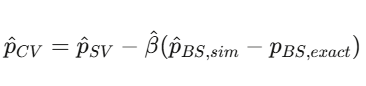
如果你在随机波动率下模拟一个二元合约 {S_T > K}(没有闭式解),可以用 Black-Scholes 的数字期权价格 p_{BS}(它有闭式解)作为控制变量(control variate):
def stratified_binary_mc(S0, K, sigma, T, J=10, N_total=100_000):
    """
    Stratified MC for binary contract pricing.
    Strata defined by quantiles of the terminal price distribution.
    """
    n_per_stratum = N_total // J
    estimates = []

    for j in range(J):
        # Uniform draws within stratum [j/J, (j+1)/J]
        U = np.random.uniform(j/J, (j+1)/J, n_per_stratum)
        Z = norm.ppf(U)
        S_T = S0 * np.exp((-0.5*sigma**2)*T + sigma*np.sqrt(T)*Z)
        stratum_mean = (S_T > K).mean()
        estimates.append(stratum_mean)

    # Each stratum has weight 1/J
    p_stratified = np.mean(estimates)
    se_stratified = np.std(estimates) / np.sqrt(J)

    return p_stratified, se_stratified

p, se = stratified_binary_mc(S0=100, K=105, sigma=0.20, T=30/365)
print(f"Stratified estimate: {p:.6f} ± {se:.6f}")
分而治之
把概率空间划分为 J 个分层(strata),在每一层内采样,再组合。按照全方差定律,方差总是 ≤ 朴素 MC;最大增益来自Neyman 分配:nj∝ωjσj(对方差高的分层更多采样)。
把三者叠起来
在每一层里用对偶变量(antithetic variates),再叠加控制变量校正,你往往能比朴素 MC 把方差降低 100–500 倍。这在生产里不是可选项,这是入场门槛。
第六部分:建模相关矩阵做不到的东西
分层贝叶斯模型通过共享的全国摆动参数,隐式地编码了相关性。
但尾部相关性(tail dependence)呢——那种在极端情况下的共振,在简单线性相关里根本看不出来?
2008 年,高斯 copula 未能刻画尾部相关性,是全球金融危机的重要成因之一。在预测市场里,同样的问题也会出现:当一个摇摆州给出意外结果时,所有摇摆州一起翻转的概率,要远高于高斯 copula 的预测。
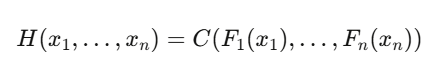
Sklar 定理
其中 C 是 copula(纯粹的依赖结构),F_i 是边缘分布的 CDF。你可以分别建模每个市场的边缘行为,然后用一个能刻画依赖(包括尾部)的 copula 把它们“粘”在一起。
尾部相关性问题
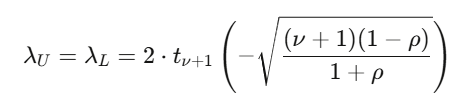
高斯 copula:尾部相关性 λU=λL=0。极端共同波动被建模为零概率。
这对相关联的预测市场来说是灾难性错误。
Student-t copula
import numpy as np
from collections import deque

class PredictionMarketABM:
    """
    Agent-based model of a prediction market order book.

    Agent types:
    - Informed: know the true probability, trade toward it
    - Noise: random trades
    - Market maker: provides liquidity around current price
    """
    def __init__(self, true_prob, n_informed=10, n_noise=50, n_mm=5):
        self.true_prob = true_prob
        self.price = 0.50  # initial price
        self.price_history = [self.price]

        # Order book (simplified as bid/ask queues)
        self.best_bid = 0.49
        self.best_ask = 0.51

        # Agent populations
        self.n_informed = n_informed
        self.n_noise = n_noise
        self.n_mm = n_mm

        # Track metrics
        self.volume = 0
        self.informed_pnl = 0
        self.noise_pnl = 0

    def step(self):
        """One time step: randomly select an agent to trade."""
        total = self.n_informed + self.n_noise + self.n_mm
        r = np.random.random()

        if r < self.n_informed / total:
            self._informed_trade()
        elif r < (self.n_informed + self.n_noise) / total:
            self._noise_trade()
        else:
            self._mm_update()

        self.price_history.append(self.price)

    def _informed_trade(self):
        """Informed trader: buy if price < true_prob, sell otherwise."""
        signal = self.true_prob + np.random.normal(0, 0.02)  # noisy signal

        if signal > self.best_ask + 0.01:  # buy
            size = min(0.1, abs(signal - self.price) * 2)
            self.price += size * self._kyle_lambda()
            self.volume += size
            self.informed_pnl += (self.true_prob - self.best_ask) * size
        elif signal < self.best_bid - 0.01:  # sell
            size = min(0.1, abs(self.price - signal) * 2)
            self.price -= size * self._kyle_lambda()
            self.volume += size
            self.informed_pnl += (self.best_bid - self.true_prob) * size

        self.price = np.clip(self.price, 0.01, 0.99)
        self._update_book()

    def _noise_trade(self):
        """Noise trader: random buy/sell."""
        direction = np.random.choice([-1, 1])
        size = np.random.exponential(0.02)
        self.price += direction * size * self._kyle_lambda()
        self.price = np.clip(self.price, 0.01, 0.99)
        self.volume += size
        self.noise_pnl -= abs(self.price - self.true_prob) * size * 0.5
        self._update_book()

    def _mm_update(self):
        """Market maker: tighten spread toward current price."""
        spread = max(0.02, 0.05 * (1 - self.volume / 100))
        self.best_bid = self.price - spread / 2
        self.best_ask = self.price + spread / 2

    def _kyle_lambda(self):
        """Price impact parameter."""
        sigma_v = abs(self.true_prob - self.price) + 0.05
        sigma_u = 0.1 * np.sqrt(self.n_noise)
        return sigma_v / (2 * sigma_u)

    def _update_book(self):
        spread = self.best_ask - self.best_bid
        self.best_bid = self.price - spread / 2
        self.best_ask = self.price + spread / 2

    def run(self, n_steps=1000):
        for _ in range(n_steps):
            self.step()
        return np.array(self.price_history)

# --- Simulation ---
np.random.seed(42)

# Scenario: true probability is 0.65, market starts at 0.50
sim = PredictionMarketABM(true_prob=0.65, n_informed=10, n_noise=50, n_mm=5)
prices = sim.run(n_steps=2000)

print("Agent-Based Prediction Market Simulation")
print(f"True probability:   {sim.true_prob:.2f}")
print(f"Starting price:     0.50")
print(f"Final price:        {prices[-1]:.4f}")
print(f"Price at t=500:     {prices[500]:.4f}")
print(f"Price at t=1000:    {prices[1000]:.4f}")
print(f"Total volume:       {sim.volume:.1f}")
print(f"Informed P&L:       ${sim.informed_pnl:.2f}")
print(f"Noise trader P&L:   ${sim.noise_pnl:.2f}")
print(f"Convergence error:  {abs(prices[-1] - sim.true_prob):.4f}")
在 ν=4、ρ=0.6 时,尾部相关性大约是 0.18——也就是:在某个合约出现极端结果的条件下,约有 18% 的概率会发生极端共同波动。高斯模型会给出 0%。
Clayton copula:只有下尾相关性(λL=2^−1/θ)。当一个预测市场崩盘,其他市场会跟着崩;没有上尾相关性。
Gumbel copula:只有上尾相关性(λU=2−2^1/θ)。相关的正向结算。
模拟相关的预测市场结果
def rare_event_IS(S0, K_crash, sigma, T, N_paths=100_000):
    """
    Importance sampling for extreme downside binary contracts.

    Example: P(S&P drops 20% in one week)
    """
    K = S0 * (1 - K_crash)  # e.g., 20% crash threshold

    # Original drift (risk-neutral)
    mu_original = -0.5 * sigma**2

    # Tilted drift: shift the mean toward the crash region
    # Choose mu_tilt so the crash threshold is ~1 std dev away instead of ~4
    log_threshold = np.log(K / S0)
    mu_tilt = log_threshold / T  # center the distribution on the crash

    Z = np.random.standard_normal(N_paths)

    # Simulate under TILTED measure
    log_returns_tilted = mu_tilt * T + sigma * np.sqrt(T) * Z
    S_T_tilted = S0 * np.exp(log_returns_tilted)

    # Likelihood ratio: original density / tilted density
    log_returns_original = mu_original * T + sigma * np.sqrt(T) * Z
    log_LR = (
        -0.5 * ((log_returns_tilted - mu_original * T) / (sigma * np.sqrt(T)))**2
        + 0.5 * ((log_returns_tilted - mu_tilt * T) / (sigma * np.sqrt(T)))**2
    )
    LR = np.exp(log_LR)

    # IS estimator
    payoffs = (S_T_tilted < K).astype(float)
    is_estimates = payoffs * LR

    p_IS = is_estimates.mean()
    se_IS = is_estimates.std() / np.sqrt(N_paths)

    # Compare with crude MC
    Z_crude = np.random.standard_normal(N_paths)
    S_T_crude = S0 * np.exp(mu_original * T + sigma * np.sqrt(T) * Z_crude)
    p_crude = (S_T_crude < K).mean()
    se_crude = np.sqrt(p_crude * (1 - p_crude) / N_paths) if p_crude > 0 else float('inf')

    return {
        'p_IS': p_IS, 'se_IS': se_IS,
        'p_crude': p_crude, 'se_crude': se_crude,
        'variance_reduction': (se_crude / se_IS)**2 if se_IS > 0 else float('inf')
    }

result = rare_event_IS(S0=5000, K_crash=0.20, sigma=0.15, T=5/252)
print(f"IS estimate:    {result['p_IS']:.6f} ± {result['se_IS']:.6f}")
print(f"Crude estimate: {result['p_crude']:.6f} ± {result['se_crude']:.6f}")
print(f"Variance reduction factor: {result['variance_reduction']:.1f}x")
这正是 2008 年高斯 copula 失败的根本原因;对预测市场组合来说,它也会再次失败。
ν=4 的 t-copula 往往会显示:极端联合结果的概率比高斯模型高出 2–5 倍。
如果你在交易相互相关的预测市场合约却不建模尾部相关性,那么你就在运行一个组合——它会在最关键的情景里精准爆炸。
藤 copula(Vine Copula)
当合约维度 d>5 时,仅靠二元 copula 不够。藤 copula把 d 维依赖分解为 d(d−1)/2 个二元条件 copula,并以树结构组织:
-
C-vine(星型):一个中心事件驱动一切(例如:总统胜负 -> 所有政策市场)
-
D-vine(链型):顺序依赖(例如:初选结果流向大选)
-
R-vine(一般图):最大灵活性
按 ∣τKendall∣ 构建最大生成树,用 AIC 选择 pair-copula 族,顺序估计。实现:pyvinecopulib(Python)、VineCopula(R)。
第七部分:基于主体的仿真
到目前为止,我们都假设你知道数据生成过程,只需要把它模拟出来即可。
但预测市场由异质主体构成——知情交易者、噪声交易者、做市商、以及机器人。它们的互动会产生涌现的动力学,任何闭式的 SDE 都捕捉不到。
零智能的启示
即便每一个交易者都完全不理性,市场也仍然可能是有效的。
Gode & Sunder(1993)证明:零智能主体——仅在预算约束下随机下单的交易者——在连续双向竞价中也能实现接近 100% 的配置效率。
Farmer、Patelli & Zovko(2005)把这一结果扩展到了限价订单簿。
这解释了伦敦证券交易所横截面价差变化的 96%。一个参数。96%。
基于主体的预测市场模拟器
import numpy as np

def simulate_binary_contract(S0, K, mu, sigma, T, N_paths=100_000):
    """
    Monte Carlo simulation for a binary contract.

    S0:    Current asset price
    K:     Strike / threshold
    mu:    Annual drift
    sigma: Annual volatility
    T:     Time to expiry in years
    N_paths: Number of simulated paths
    """
    # Simulate terminal prices via GBM
    Z = np.random.standard_normal(N_paths)
    S_T = S0 * np.exp((mu - 0.5 * sigma**2) * T + sigma * np.sqrt(T) * Z)

    # Binary payoff
    payoffs = (S_T > K).astype(float)

    # Estimate and confidence interval
    p_hat = payoffs.mean()
    se = np.sqrt(p_hat * (1 - p_hat) / N_paths)
    ci_lower = p_hat - 1.96 * se
    ci_upper = p_hat + 1.96 * se

    return {
        'probability': p_hat,
        'std_error': se,
        'ci_95': (ci_lower, ci_upper),
        'N_paths': N_paths
    }

# Example: AAPL at $195, strike $200, 20% vol, 30 days
result = simulate_binary_contract(S0=195, K=200, mu=0.08, sigma=0.20, T=30/365)
print(f"P(AAPL > $200) ≈ {result['probability']:.4f}")
print(f"95% CI: ({result['ci_95'][0]:.4f}, {result['ci_95'][1]:.4f})")
价格收敛得有多快取决于知情交易者与噪声交易者的比例、做市商价差对信息流的响应方式,以及为什么知情交易者能在噪声交易者的损失上实现盈利。
第八部分:生产级技术栈
下面是完整系统——从市场数据到交易执行:
- LAYER 1: 数据接入
- 来自 Polymarket CLOB API 的 WebSocket 推送(实时价格、成交量)
- 新闻/民调数据流(经 NLP 处理为概率信号)
-
链上事件数据(Polygon)
-
LAYER 2: 概率引擎
- 分层贝叶斯模型(Stan/PyMC)给出州级后验
- 粒子滤波:对新观测进行实时更新
- 跳跃-扩散 SDE 的路径仿真用于风险管理
-
集成(Ensemble):对模型输出做加权平均
-
LAYER 3: 依赖建模
- 藤 copula:合约之间的两两依赖
- 因子模型:共享的全国/全球风险因子
-
用 t-copula 估计尾部相关性
-
LAYER 4: 风险管理
- 基于 EVT 的 VaR 与期望短缺(Expected Shortfall)
- 反向压力测试:找出最坏情景
- 相关性压力:如果州与州的相关性突然飙升会怎样?
-
流动性风险:监控订单簿深度
-
LAYER 5: 监控
- 追踪布里尔分数(我们校准了吗?)
- P&L 归因(哪个模型组件贡献了价值?)
- 回撤告警
- 模型漂移检测
参考文献
-
Dalen(2025)。《走向预测市场的 Black-Scholes》。arXiv:2510.15205
-
Saguillo 等(2025)。《解开概率森林:预测市场中的套利》。arXiv:2508.03474
-
Madrigal-Cianci 等(2026)。《作为贝叶斯逆问题的预测市场》。arXiv:2601.18815
-
Farmer、Patelli & Zovko(2005)。《零智能的预测力》。PNAS
-
Gode & Sunder(1993)。《零智能交易者市场的配置效率》。JPE
-
Kyle(1985)。《连续竞价与内幕交易》。Econometrica
-
Glosten & Milgrom(1985)。《买价、卖价与成交价》。JFE
-
Hoffman & Gelman(2014)。《No-U-Turn 采样器》。JMLR
-
Merton(1976)。《当标的股票收益不连续时的期权定价》。JFE
-
Linzer(2013)。《总统选举的动态贝叶斯预测》。JASA
-
Gelman 等(2020)。《更新后的动态贝叶斯预测模型》。HDSR
-
Aas、Czado、Frigessi & Bakken(2009)。《多元依赖的 Pair-Copula 构造》。Insurance: Mathematics and Economics
-
Wiese 等(2020)。《Quant GANs:金融时间序列的深度生成》。Quantitative Finance