大语言模型究竟是如何工作的

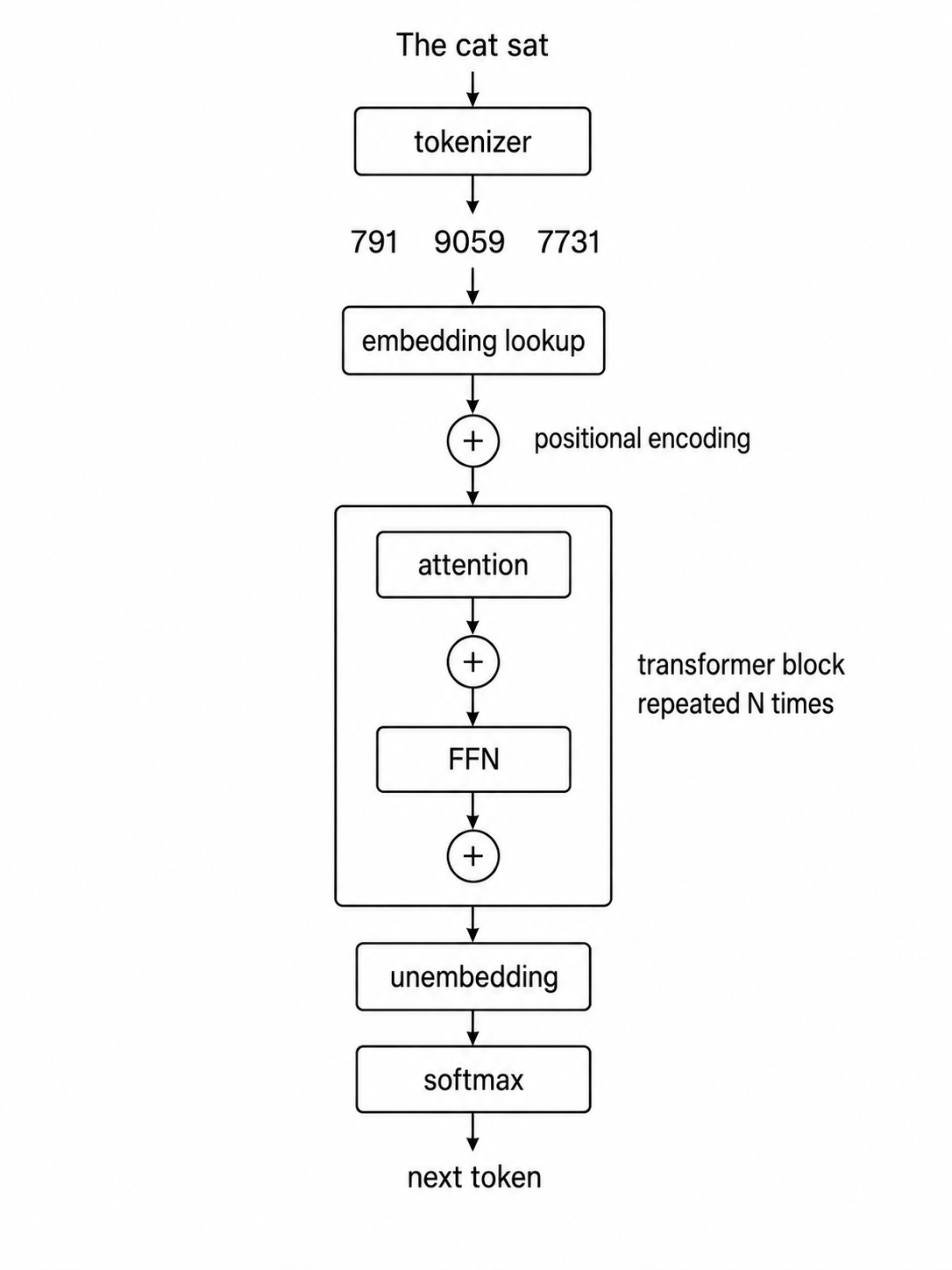
Monday. June 01, 2026 - 26 mins This post is a walkthrough of how LLMs work. Modern LLMs are mostly built by stacking transformer blocks over and over, so understanding the transformer machinery gets you most of the way there.

I’ll cover the core mechanisms inside modern transformer-based LLMs, without all that sticky math stuff. Don’t get me wrong, you should learn the math, but this can serve as an introduction.

Most modern LLMs share the same transformer-family skeleton. The differences come from what each one was trained on, the scale and configuration choices, and the post-training done on top. By the end, you should be able to read many modern LLM papers or model cards and know which piece of the architecture each section is talking about.

Here’s the path:

1. Tokens, how a string of text becomes a sequence of integers
2. Embeddings, how those integers get meaning
3. Positional encoding, how the model knows what order the tokens came in
4. Attention, how tokens share information with each other
5. Multi-head attention, how the model tracks many kinds of relationships at once
6. The feed-forward network, where a large share of the model’s stored structure lives
7. The residual stream and layer normalization, what makes deep stacks trainable
8. Predicting the next token, what the model actually outputs and how the generation loop works
9. Architecture vs trained weights, what’s broadly shared across modern LLMs, and what’s different

Tiny explainers appear throughout so anyone can follow along, regardless of background.

Tokenization

Models don’t read text directly. They read integer IDs. The step that converts your prompt into a sequence of those integers.

That conversion step is called tokenization. A tokenizer takes a string and produces a sequence of integers, where each integer points to an entry in a fixed vocabulary. Modern LLM vocabularies usually contain tens of thousands to a few hundred thousand entries.

Tiny explainer: token ID

A token ID is the integer the model uses for one vocabulary entry. The model works with the number, not the written word itself.

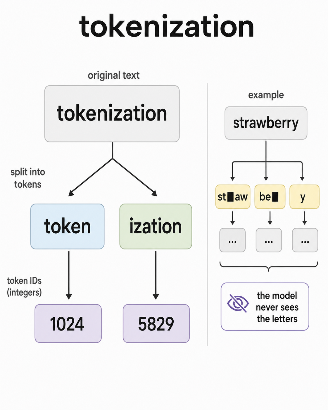
Tokens aren’t usually whole words. They’re usually subword pieces. The word “tokenization” might split into [“token”, “ization”]. The word “running” might split into [“run”, “ning”]. The reason is efficiency. Whole-word vocabularies are too big and don’t generalize to new words. Character-level vocabularies are too small and force the model to learn even the simplest patterns from scratch. Subword tokenization sits in the middle. The most common pieces become single tokens, and rare or novel words get composed from smaller pieces.

Tiny explainer: vocabulary

The vocabulary is the tokenizer’s fixed list of pieces. Each piece has an ID, and the model can only directly receive IDs from that list.

The trade-off shows up in places people don’t expect. The classic example: ask an LLM how many R’s are in “strawberry.” LLMs used to get it wrong. That’s not the model failing at counting. It’s the model not operating on letters directly, only token IDs that happen to spell out a word a human would split letter by letter.

Different model families use different tokenizers. GPT models use Byte Pair Encoding variants. SentencePiece is common in LLaMA-style models. The choice matters for compute (fewer tokens means less work) and for things like multilingual coverage, but the basic shape is the same. Text in, integers out.

Now that the prompt is a sequence of integers, the next step is to give those integers meaning.

Embeddings

A token ID like 1024 is just a row index. It doesn’t mean anything by itself. The thing that gives it meaning is a giant table called the embedding matrix.

Every model has one. It has one row per entry in the vocabulary, and each row is a long vector of numbers. The length of each row is the model’s hidden size. In many 7B-class models, that means 4,096 numbers per token. Larger models usually use wider vectors.

Tiny explainer: vector

A vector is a list of numbers. In a transformer, each token becomes a vector so the model can do math with it.

When the tokenizer hands the model an integer, the model looks up that row and uses the vector instead. That vector is the token’s embedding. It’s the model’s representation of what that token “means,” learned during training.

Tiny explainer: embedding matrix

The embedding matrix is a lookup table. Token ID in, learned vector out.

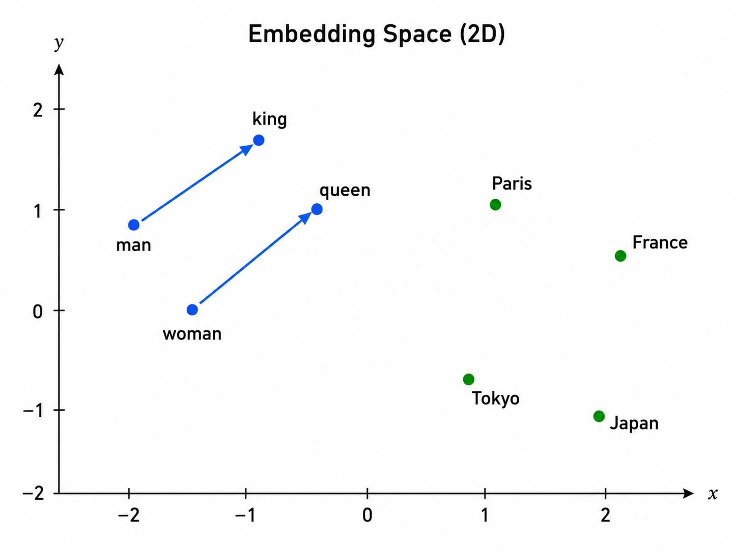
The interesting property of these embeddings is that semantically similar tokens end up with similar vectors. The vector for “king” is close in space to the vector for “queen,” and the vector for “Paris” is close to “France.” None of this is hard-coded. It emerges from training on enough text, and the model learns these positions because they let it predict text well.

You can do arithmetic on embeddings and it sometimes works. The famous example is king − man + woman ≈ queen. The geometry of embedding space carries real semantic structure, even though nobody told the model to build it that way.

Worth being clear on: at this stage every token has been replaced by its embedding, but the embedding alone says nothing about where the token sits in the sequence. The vector for “dog” is the same vector whether “dog” is the first word in your prompt or the fifth. That’s a problem.

That’s the gap positional encoding fills.

Positional encoding

Plain self-attention doesn’t have a built-in representation of word order. Without some positional signal, it has no direct way to know that “dog” came before “bites” instead of after it.

Word order changes meaning. So the model needs another piece. It needs a way to inject the position of each token into the math.

Tiny explainer: positional encoding

Positional encoding is how the model gets order information. It tells the model where each token sits in the sequence.

The original transformer paper (Vaswani et al. 2017) did this by giving each position its own pattern of numbers and adding it directly to each token’s embedding before any other processing. Position 1 had one pattern, position 5 had a different pattern, position 100 had another. The patterns came from sine and cosine waves at different frequencies. Now the embedding for “dog” at position 1 was different from the embedding for “dog” at position 5, just because the position pattern added to it was different.

That worked, and sinusoidal encodings were chosen partly because they can extrapolate beyond the exact sequence lengths seen during training. But additive position schemes still had two problems that became important as models scaled up.

First, the embedding had to carry both meaning and position in the same set of numbers. There’s only so much you can pack in.

Second, learned absolute position embeddings in particular don’t generalize cleanly. If you trained on prompts up to 2,048 tokens long, the model never saw position 5,000 during training, and the embedding for that position was not learned in the same way.

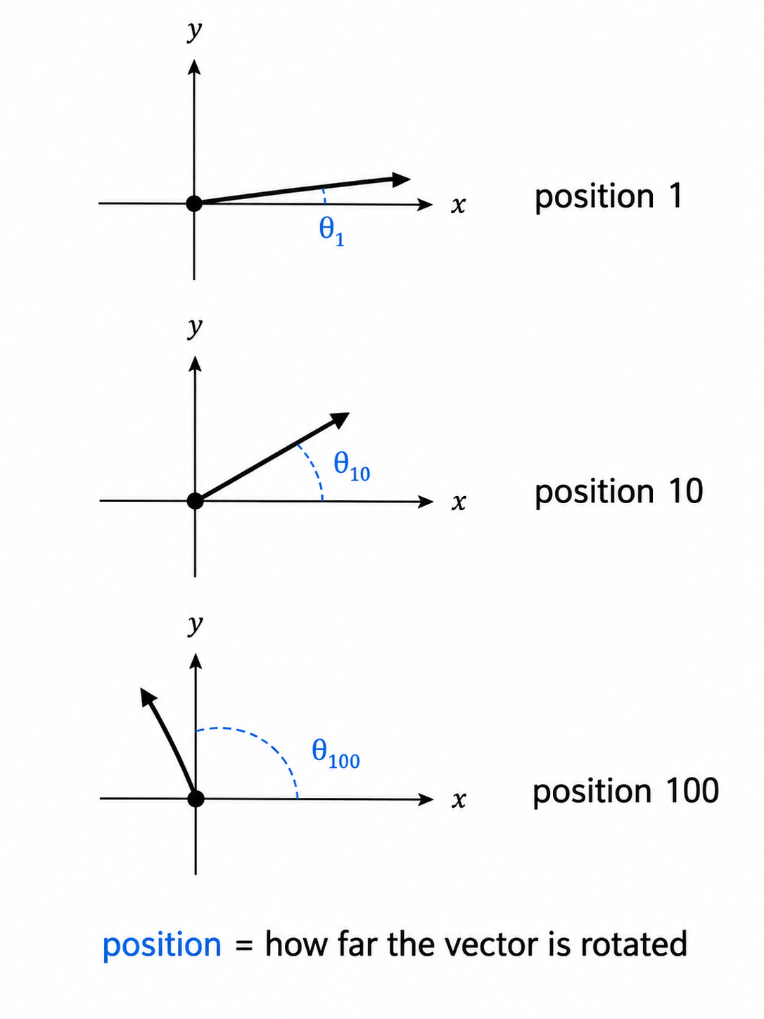
Modern models mostly use a different scheme called Rotary Position Embeddings (RoPE), introduced by Su et al. in 2021 and now used in LLaMA, Mistral, Gemma, Qwen, and most other open-weight families. The intuition: instead of adding position info to each token’s vector, RoPE rotates the Query and Key vectors by an angle that depends on the token’s position. A token at position 1 gets a small turn, a token at position 100 gets a bigger turn. When two tokens are later compared during attention, what matters is the difference between their Query and Key rotations, which encodes how far apart they are.

Tiny explainer: RoPE

RoPE stands for Rotary Position Embeddings. Instead of adding a position vector, it rotates Query and Key vectors so relative distance shows up during attention.

The practical advantages are real. RoPE encodes relative position naturally (which is closer to what attention actually wants). It generalizes better to longer contexts. And it doesn’t add new parameters to the model.

Even with good positional encoding, modern LLMs have a documented “lost in the middle” problem (Liu et al. 2023). They use information at the start and end of long prompts more reliably than information buried in the middle. That’s why prompt engineering tips like “put important context first” or “repeat key info at the end” actually help. The model isn’t using every part of your prompt equally well.

With token meaning and position both encoded, the next question is how do tokens actually exchange information?

Attention

This is the mechanism that gave the architecture its name. Attention.

Inside every transformer layer, attention does one thing. It lets each token look at the other tokens it is allowed to see and decide which ones matter for what comes next.

It does this by giving each token three roles at once. Each token gets transformed into three new vectors, called Query, Key, and Value (Q, K, V).

Tiny explainer: Q, K, V

Query means “what am I looking for,” Key means “what do I match with,” and Value is the information that gets copied when the match is strong.

• The Query asks, “what am I looking for from other tokens?”
• The Key says, “this is what I offer to tokens looking at me.”
• The Value carries, “this is what gets passed along when a match happens.”

The same token plays all three roles at the same time. The Q, K, V transformations are learned matrices, so the model figures out during training what each token should look for and what it should offer.

Matching happens through a similarity score. Each token’s Query is compared against the Key of each token it is allowed to see, using a scaled dot product. Intuitively, this measures how much the two vectors line up. The scaling keeps the numbers stable before softmax.

Tiny explainer: dot product

A dot product is a simple way to score how aligned two vectors are. Higher alignment means a stronger match.

The match scores then get turned into weights using softmax. Softmax takes any set of numbers and turns them into a probability-like distribution that sums to 1. Tokens with higher match scores get higher weights, and the weights are then used to take a weighted average of the value vectors.

Tiny explainer: softmax

Softmax turns raw scores into weights that add up to 1. Big scores get big weights, small scores get small weights.

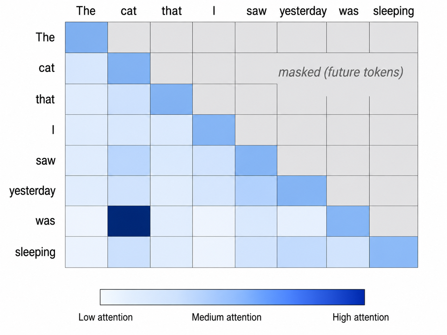
An example. Consider the sentence “The cat that I saw yesterday was sleeping.” When the model processes “was,” it needs to figure out what’s doing the sleeping. The Query vector for “was” gets compared against the Key vectors of the tokens it is allowed to see. The dot product with “cat” is high, because the model has learned that verbs like “was” need a subject and that subjects like “cat” produce Key vectors that line up well. The dot product with “yesterday” is low. Softmax turns those scores into weights, “cat” gets a high weight, “yesterday” gets a low one. The model then takes a weighted sum of the corresponding value vectors, so the value for “cat” dominates the result. The new representation of “was” is now mostly shaped by the value of “cat.” That’s how a token several positions back becomes the referent.

There’s a constraint specific to GPT-style language models, which is that they generate text left to right. A token at position 5 is only allowed to attend to positions 1 through 5. It cannot attend to tokens at positions 6, 7, 8, because those haven’t been generated yet. This is called causal masking. The implementation is simple: future tokens get match scores so low they end up with effectively zero weight after softmax.

Tiny explainer: causal masking

Causal masking hides future tokens. It keeps a decoder-only language model from looking ahead while predicting the next token.

One of the most interesting findings in interpretability research is about specialized attention heads called induction heads, found by Anthropic in 2022. These heads learn to spot patterns of the form “A B … A” in the prompt and predict that B comes next. When the model sees “A” the second time, the induction head looks back to where “A” appeared before, sees what came after, and copies that. They’re one of the clearest known mechanisms behind in-context learning, the ability of an LLM to pick up a pattern from your prompt and continue it.

Tiny explainer: induction head

An induction head is an attention head that notices repeated patterns in the prompt and helps continue them.

Attention has one big cost. In full attention, each token compares against all the tokens it is allowed to see, so doubling the prompt length roughly quadruples the work. This is why long prompts are expensive to run, and why a lot of recent research is about making attention more efficient (FlashAttention, sparse attention, linear attention).

But one attention head only gives the model one learned view of those relationships.

Multi-head attention

A single attention pass gives the model one way of deciding which tokens matter to which other tokens. That’s not enough. Language has many relationships happening at the same time. Subject and verb agreement. Pronouns and the names they refer to. Long-range references between sentences. Word order and local phrases.

Multi-head attention solves this by running attention many times in parallel, with each parallel pass operating in its own smaller space. Each parallel pass is called a head.

Tiny explainer: attention head

An attention head is one independent attention pass with its own learned projections.

The part that’s often described wrong, including in plenty of tutorials. Each head doesn’t get a literal slice of the original token vector. Each head has its own learned projection matrices that map the full token vector down to its own smaller Q, K, and V vectors. So if a model has 4,096 numbers per token and 32 heads, each head usually works in a 128-dimensional space, but those 128 numbers are a learned projection of the full 4,096, not a fixed slice. Different “views” of the same token, not different chunks of it.

Each head runs its attention pass independently. Then the outputs of all the heads get concatenated and passed through a final linear layer that mixes them back into one full-size vector. The model learns that final mixing too.

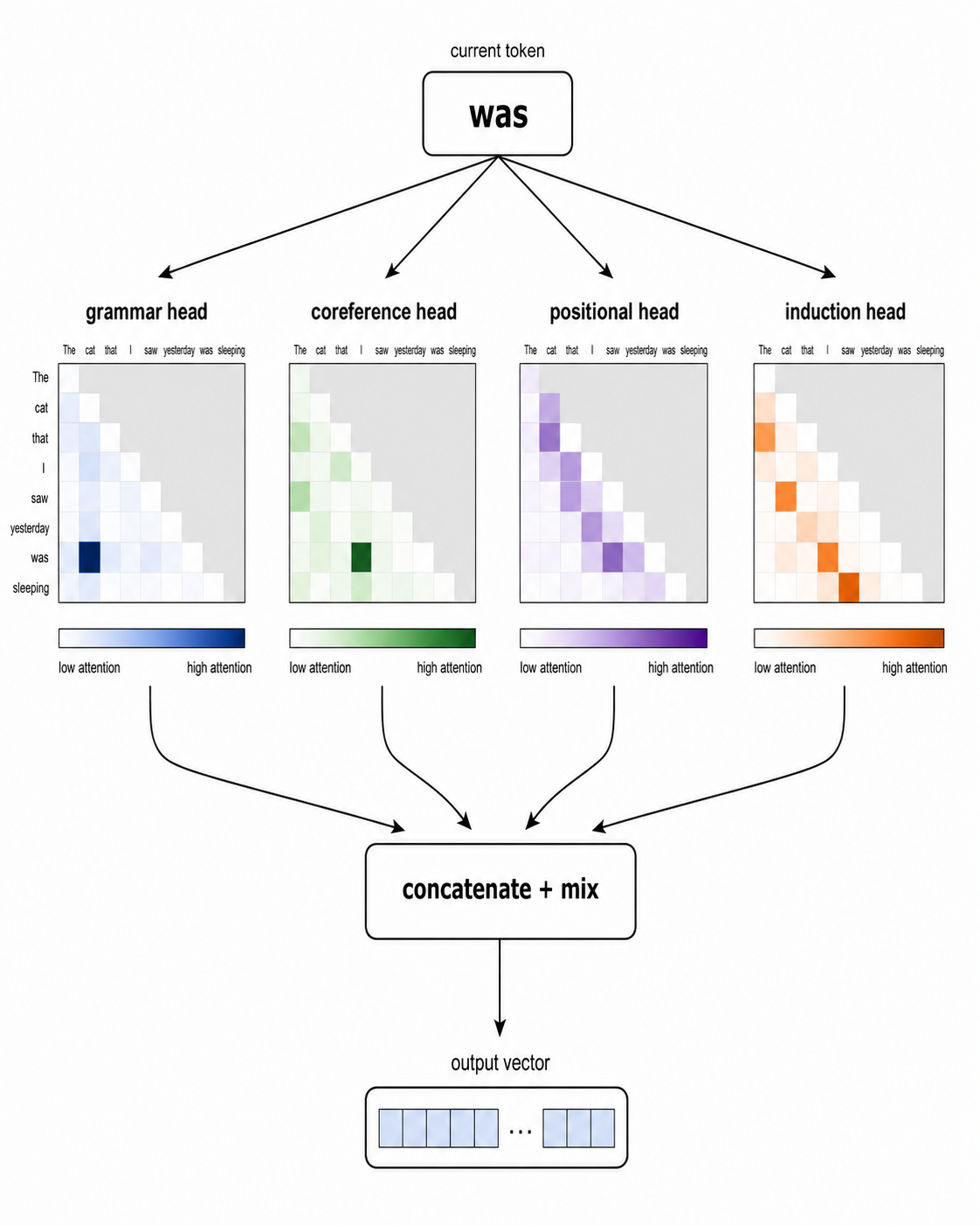
What makes this interesting is that different heads often end up partially specialized. The model is never told what each head should do. Specialization emerges naturally during training. Researchers have found heads that track grammar (linking verbs to their objects, articles to their nouns), heads that figure out which pronoun refers to which name, heads that track positional patterns, induction heads, and many more. A single transformer layer might have 32 heads. A modern frontier model has dozens of layers. So a typical LLM has thousands of attention heads in total, each adding its own learned view.

There’s a practical cost concern that drove a recent architectural change. Each head needs to keep its Key and Value vectors in memory for all the tokens already generated, so that when a new token gets generated the model doesn’t have to recompute everything from scratch. This is called the KV cache, and it’s the main memory cost of running an LLM at long context lengths.

Tiny explainer: KV cache

The KV cache stores old Key and Value vectors during generation. It saves the model from recomputing the whole prompt every time it adds a token.

Modern decoder-only LLMs mostly use a variant called Grouped-Query Attention (GQA). Instead of every head having its own keys and values, groups of heads share the same key and value heads. LLaMA-2 70B has 64 query heads but only 8 key/value heads. Mistral 7B has 32 query heads and 8 key/value heads. The result is nearly the same accuracy as full multi-head attention but with much less memory pressure and inference cost.

Tiny explainer: GQA

Grouped-Query Attention lets multiple query heads share fewer key/value heads. That cuts KV-cache memory while keeping many query views.

Feed-forward network

After attention finishes mixing information between tokens, every layer has a second step that nobody talks about as much. The feed-forward network.

Where attention is about tokens talking to each other, the feed-forward network is about each token, on its own, doing more processing. It runs on every token’s vector independently, with no cross-token mixing.

The feed-forward network does three things in order:

1. Expand the token’s vector to a larger size (the original transformer used 4x, while modern SwiGLU models often use different expansion sizes).
2. Apply a non-linear function.
3. Compress the vector back down to its original size.

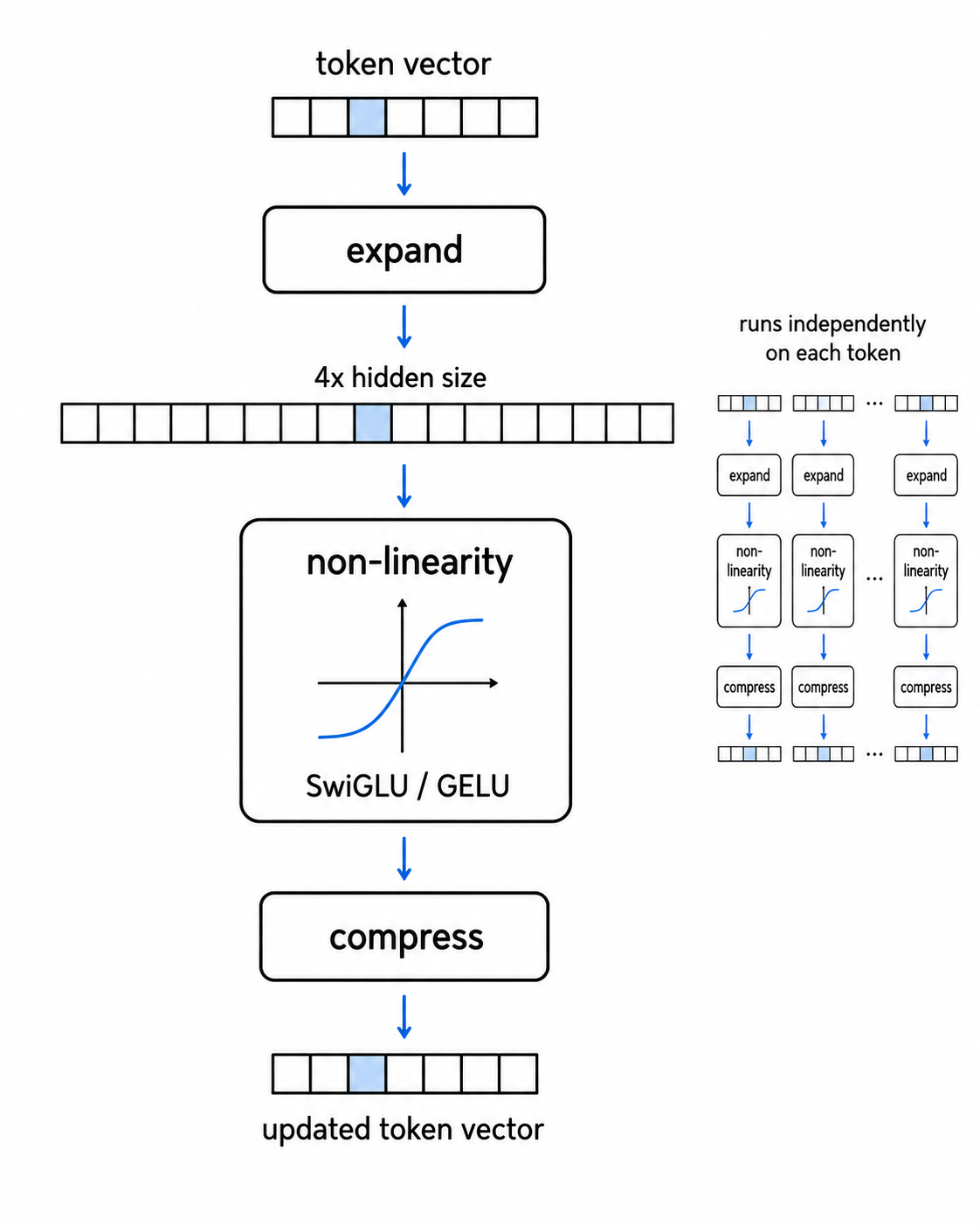
That non-linear step in the middle is doing something specific that’s worth understanding. A non-linearity is a function that bends its input. The simplest one, ReLU, outputs zero for any negative number and passes positive numbers through unchanged.

Tiny explainer: non-linearity

A non-linearity is a function that prevents the network from collapsing into one big linear transformation.

Without it, the FFN would just be two linear layers stacked together, and stacking pure linear math collapses. Two linear layers in a row are mathematically equivalent to a single linear layer, and a hundred linear layers in a row are still equivalent to one. The non-linearity is what stops that collapse, and it’s the reason the FFN can do something richer than a single matrix multiplication.

The original transformer used ReLU. GPT and BERT moved to GELU. Modern models like LLaMA, Mistral, and PaLM use SwiGLU. The expand-then-compress structure stayed the same. The non-linearity itself is what’s been iterated on.

Most of the parameters in a dense transformer model live in the FFN, not in attention. A large share of the weights sit in feed-forward layers.

And those parameters aren’t generic. They’re where much of the model’s stored factual and semantic structure lives. Researchers have found that some neurons inside the FFN are strongly associated with specific concepts or facts. One neuron might activate strongly on Eiffel-Tower-related text. Another on programming languages. Another on past-tense verbs. When a model “knows” that Paris is the capital of France, that fact is represented across FFN weights and activations in specific layers.

This stored-memory property has an interesting consequence. Researchers have figured out how to directly edit some facts in a trained model without retraining it. Methods like ROME (Rank-One Model Editing) can change “the Eiffel Tower is in Paris” to “the Eiffel Tower is in Rome” by making a targeted low-rank edit to a specific FFN weight matrix. The model then tends to generate text consistent with the edited association.

Some modern frontier models have started replacing the dense FFN with something called Mixture of Experts (MoE). Instead of one feed-forward network per layer, the model has many parallel FFNs (called experts) and a tiny router network that picks which experts process each token. Mixtral 8x7B has 8 experts per layer; only 2 are activated for any given token. The total parameter count goes up substantially, but the compute per token grows much more slowly because only a few experts run. That’s how you scale parameter count without scaling inference cost in proportion.

Tiny explainer: MoE

Mixture of Experts means the model has several feed-forward networks and routes each token through only a few of them.

Mixtral 8x7B has 46.7 billion total parameters but uses about 12.9 billion per token. This has become a common option for very large models because it lets you keep growing the parameter count without making inference cost grow in proportion.

Residual stream and layer normalization

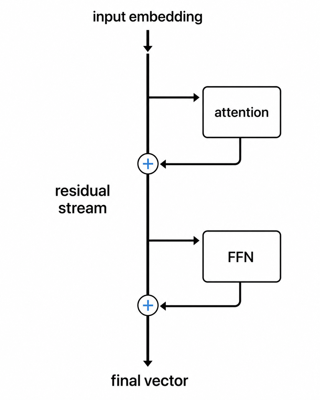
The residual stream is what makes the model “additive” instead of “replacing.” After attention runs, or after the feed-forward network runs, the result usually doesn’t replace the token’s vector. It gets added to it. Position by position. The new vector equals the old vector plus the sub-block’s output.

Tiny explainer: residual connection

A residual connection adds a block’s output back to the vector it started from. It gives information and gradients a shortcut through the network.

Across thirty or fifty or a hundred layers, each layer’s contribution accumulates instead of simply overwriting the previous vector. That running sum is called the residual stream, and it has a strange property. The original input embeddings still have a direct additive path into late layers, mixed together with every sub-block’s contribution along the way.

Residual connections weren’t invented for transformers. They came from ResNet (He et al. 2015), originally for image recognition. The motivation was that deep networks were impossible to train. The training signal got too weak (or sometimes too strong) by the time it traveled back through many layers. The model couldn’t actually learn from its own mistakes. Adding a shortcut path let the signal flow directly back from the output to the input. Suddenly you could train networks with hundreds of layers. Transformers inherited the same trick.

In modern interpretability research, the residual stream has become the central object. Every component, every attention head, every feed-forward network, even the unembedding step at the end, reads from the residual stream and writes back to it.

The second piece, layer normalization, exists for a much more practical reason. Without it, the residual stream would not stay stable. Numbers flowing through dozens of additions tend to either explode upward or collapse toward zero. Either way, training fails. Layer normalization rescales each token’s vector back into a controlled range between sub-blocks.

Tiny explainer: layer normalization

Layer normalization rescales a token vector so its numbers stay in a stable range while the model trains.

The original 2017 transformer applied normalization AFTER each sub-block (post-norm). This worked for shallow models but became harder to train reliably as depth increased. Modern transformers (GPT-2 onward, LLaMA, Mistral) commonly apply normalization BEFORE each sub-block (pre-norm). That’s one of the changes that made very deep transformers easier to train.

The function itself has also changed. Many modern open models (LLaMA, Mistral, Gemma, Phi) use a simpler variant called RMSNorm. The original layer normalization did two things at once: shift each vector toward zero, then rescale the size of the numbers. RMSNorm drops the shift step and keeps only the rescaling. Empirically, the rescaling carries most of the benefit while being cheaper to compute.

Tiny explainer: RMSNorm

RMSNorm is a cheaper normalization method that rescales vector size without subtracting the mean first.

So that’s the unglamorous machinery. Without residual connections, very deep models become much harder to train. Without layer normalization, the running sum can blow up or collapse. With both, you get models hundreds of layers deep.

Next-token prediction

After all the layers of attention and feed-forward processing finish, the model has a vector for each token in the sequence. During generation, to predict the next word, it takes the final vector of the last token only.

That last vector gets converted into one number per possible next token. If the vocabulary has 100,000 tokens, that’s 100,000 numbers. These numbers are called logits. They aren’t probabilities yet. They can be any size, positive or negative.

Tiny explainer: logits

Logits are raw scores for each possible next token. They become probabilities only after softmax.

A softmax turns those logits into the model’s probability distribution over possible next tokens. Same operation as before, different place in the model.

The model usually does not just pick the highest-probability token every time. Decoding settings control how deterministic or varied the output is. Temperature changes how sharp the distribution is. Top-k and top-p limit the choices to the most plausible next tokens. That is why the same model can feel precise in one setting and more creative in another.

Tiny explainer: temperature

Temperature controls randomness during sampling. Low temperature makes the model more conservative; high temperature makes it more varied.

Once a token is picked, it gets added to the input. The model runs the next step on the longer sequence, usually reusing the KV cache so it doesn’t recompute the whole prefix from scratch. New attention for the new token. New feed-forward. New final vector. New prediction. The loop continues until the model emits an end-of-sequence token or hits a length limit. A whole paragraph is just this loop, one token at a time.

This single objective, predicting the next token, is the core training signal for a base LLM. The base model isn’t trained on factual accuracy, conversational ability, reasoning, or coding directly. It’s trained to predict the next token in massive amounts of text. Later post-training can then tune the model for instruction following, preference, safety, and conversational behavior.

There’s been a major efficiency innovation worth knowing about. It’s called speculative decoding. A small fast model proposes several tokens ahead. The big model verifies them in parallel. If the proposed tokens are accepted under the big model’s probabilities, accept them. If not, fall back to the big model. Done correctly, the output distribution matches running the big model alone, but the loop can run much faster.

Tiny explainer: speculative decoding

Speculative decoding uses a small draft model to guess ahead, then asks the larger model to verify several guessed tokens at once.

The next-token prediction loop is the simplest part of the architecture, but it’s what makes the whole thing work.

Architecture vs trained weights

We’ve gone through the core mechanisms: tokens, embeddings, positional encoding, attention, multi-head attention, the feed-forward network, the residual stream and normalization, and the next-token loop on the output side. That’s the basic architecture in one pass.

So what’s actually different between GPT and Claude and Gemini and LLaMA? Public details vary, and the proprietary models do not publish every architectural choice. But at the level this post is covering, they broadly sit in the same transformer-family design space.

Most modern transformer-based LLMs use the same broad structure: tokenization, embeddings, positional encoding, stacked transformer layers (each with multi-head attention and a feed-forward network), residual streams, layer normalization, and next-token prediction.

What changes between models is:

1. The trained weights themselves, learned from different training data at different scales.
2. The configuration: number of layers, vocabulary size, head count, parameter count, MoE or dense.
3. The post-training: instruction tuning, learning from human feedback, safety controls applied on top of the base model.

Tiny explainer: weights

Weights are the learned numbers inside the model. Training changes those numbers until the model predicts text well.

The 2023-2025 “modern transformer” stack converged on a common set of choices across many serious frontier and open-weight models, even though different teams arrived at them independently. Pre-norm placement. RMSNorm. RoPE. SwiGLU. Grouped-Query Attention. Mixture of Experts in some of the largest models. None of these were invented at once. They accumulated over about five years of refinement on top of the original 2017 design.

Where this is going

The convergence around transformer-family architectures is unusual in machine learning history. For most of the field’s life, every problem had its own specialized network. Image recognition used one kind. Language used another. Audio used a third. Vision and language teams barely shared methods.

Now transformer-style models show up across language, vision, audio, and multimodal systems. The transformer absorbed a huge part of the field.

That could change. Mamba and other state-space models are credible alternatives, especially for very long sequences. Hybrid architectures are being explored. Mixture-of-experts has already shifted what “the architecture” means at the frontier in ways that would have been considered exotic five years ago.

But the core mechanisms in this post (tokens, embeddings, positional encoding, attention, the feed-forward network, the residual stream and normalization, and next-token prediction) are the durable parts. Even when the architecture changes, these are the problems any sequence model has to solve in some form.

If you’ve made it this far, you can read many modern transformer papers or model cards and know which piece each section is talking about. That’s the goal.

Feedback is extremely welcome. If any of this interests you, please reach out on X. I love making new friends.

Feedback is extremely welcome. If any of this interests you, please reach out on X. I love making new friends.