返回列表
🧠 阿头学

MoE推理架构的解耦经济学与“Token工厂”范式

MoE推理必须将Prefill、Midfill与Decode解耦为异构Worker池,并以高带宽移动替代大容量堆砌,否则长上下文Agent场景将陷入算力闲置与延迟雪崩的双重陷阱。
打开原文 ↗

2026-09-22 原文链接 ↗
阅读简报
双语对照
完整翻译
原文
讨论归档

核心观点

  • 操作模式必须按算术强度解耦:Prefill与Midfill属计算密集型且极易形成专家批次,Decode属内存密集型且专家共享率极低,强行混合调度必然导致算力与带宽相互拖累。
  • KV Cache应转为不可变Blob的共享存储:将热状态剥离出昂贵HBM并下沉至CPU内存与并行文件系统,能彻底打破长上下文推理的内存墙,但跨节点传输的网络抖动风险被严重低估。
  • Decode阶段的小批次经济优于盲目扩吞吐:MoE架构下Decode的KV读取具有强私有性,扩大Batch Size仅能带来边际吞吐提升却会成倍恶化交互延迟,硬件设计必须优先保障1-5的小批次低延迟。
  • 分离式架构的运维成本与容错盲区未解:多池异构调度虽能提升理论利用率,但KV状态重建开销、Worker冷启动延迟及集群碎片化将直接吞噬理论收益,聚合式“全能芯片”在特定场景下仍具不可替代性。

跟我们的关联

  • 对 Neta(AI架构):意味着推理集群采购逻辑需从“堆算力”转向“带宽与存储分层”,下一步应基于KV内存交叉点公式重新评估GPU显存配置,并优先验证Prefill/Decode分离调度器的生产稳定性。
  • 对 ATou(Agent产品):意味着上下文管理策略直接决定底层算力成本,下一步必须将Agent历史重构为“状态快照+增量更新”的不可变Blob架构,避免全量上下文加载击穿推理内存墙。
  • 对 Uota(硬件投资):意味着HBM容量军备竞赛的边际收益已见顶,下一步应重点押注高带宽内存与低延迟纵向扩展网络供应商,警惕单纯堆砌容量的硬件路线。

讨论引子

  • 在MoE长上下文场景下,Decode阶段的最佳Batch Size被压缩至1-5,这是否意味着当前以“高吞吐”为卖点的推理芯片将面临商业逻辑失效?
  • 分离式“Token工厂”架构虽能提升理论MFU,但跨池KV传输的网络延迟与状态重建成本在真实生产环境中究竟会吞噬多少收益?
  • 若线性注意力或激进KV压缩技术在未来两年内突破,本文基于全注意力假设推导的“内存墙”与“分离必要性”是否会彻底崩塌?

混合专家模型现已广泛应用于前沿模型中,它不仅改变了服务的结构,也改变了有效推理的经济学。它的作用远不止增加参数量。它改变了每个 token 激活哪些张量,哪些数据必须保持紧密聚合,哪些传输需要强大的本地带宽,哪些可以容忍较弱的网络连接,以及内存移动、存储和调度如何为有效吞吐量做出贡献。

最佳的切入点是整体服务。推理运行在一个由编排层(如 NVIDIA Dynamo、Mooncake 或自定义调度器)协调的集群内。这些编排层与 vLLM 或 SQlang 等推理服务器紧密协作,而这些服务器本身也具备各自的编排特性。本文不会深入探讨如何使用编排软件或该如何选择的细节。本文旨在概述您可能使用的各种特性的流程及其背后的原因。

用户(或其代理)通过请求开始对话,并在收到回答后可能继续发起更多请求。这种“请求-回答”过程构成一个“轮次”。在现代 AI 系统中,用户通常在客户端应用程序(无论是 GUI 还是命令行界面)中运行,而从 AI 返回的部分回答会被该应用程序拦截作为其执行的指令,例如编辑您的代码或就人力资源问题搜索公司指南。

AI 系统也可以在其数据中心内自行完成其中某些操作,例如搜索网络。这些拦截工具操作的结果也会作为请求返回给 AI,从而产生更多轮次。服务器会维护一个上下文(通常被称为 KV cache 或直接称为 cache),它是整个会话的精华,使得来自用户或工具的每个新请求都能被正确解释,以实现整体的向前推进。当用户启动代理执行长时间运行的任务时,每小时可能会产生数千个轮次。对话也可以暂停,并在几小时甚至几天后恢复。

当请求到达推理服务器时,编排器会将其放入队列,随后将连同系统提示词和对话中先前轮次的上下文一起输入到 input-fill worker 中。然后,该查询被转换为新的上下文并附加到对话中。接着,这个新的上下文状态被移动到 decode worker。Decode worker 会反复读取累积的状态,生成回答 token,而这些回答 token 也会被附加到对话状态中。这个过程可能会在工具、代理、用户以及进一步的 input-fill 工作之间循环。在 GPU 上运行的模型 worker 只是这个 token 工厂的一部分;存储、网络和编排将它的各个阶段连接起来。

在 worker 内部,有四种操作模式从一开始就值得区分:

Prefill,即初始的新 token 块被一起处理的阶段。

Midfill,即延续请求被附加到现有缓存上下文中的阶段。

Decode attention,即使用上下文生成新 token 基础的阶段。

Decode experts,即每个基础新 token 由从大量可能的专家中选出的部分专家进行细化的阶段。

这些模式对计算、内存和网络提出了不同的要求。Prefill 和 midfill 密切相关,Prefill 可以看作是先前上下文为零的 Midfill。然而,Prefill 是一种常见的特殊情况,对应于经典的“聊天机器人”使用等一次性查询,其优化方式可能与 Midfill 略有不同。Prefill 达到了很高的算术强度(Arithmetic Intensity,即计算量与数据移动量的比率),并且不需要等待上下文定位和读取。Midfill 从用于先前状态的现有 KV cache 开始,并附加新的请求输入序列。这通常具有比 prefill 更温和的算术强度,因为每个 token 对应的新 token 更少,而需要移动的现有数据更多。

Decode attention 和 decode expert 工作通常具有较低的算术强度,因为与先前上下文或专家权重相比,新 token 很少,而在 decode 状态下这些权重是需要移动的数据。同时,在所有模式中,无论 token 的值如何,attention 和 expert 的张量都是相同的,因此,将一次张量读取共享给尽可能多的可排队使用的 token 是有益的,甚至是那些恰好同时运行且网络距离足够近以实现共享的、来自其他用户不相关请求的 token。将这四种模式视为相同的工作负载,会丧失 MoE 模型在 不同强度和不同共享模式方面所提供的许多结构优势。

在本文中,我们将分别讨论这 4 个阶段,有时会假设它们是分离的。在聚合(模型保留在一个服务器上,随着请求在各个阶段之间推进而重新配置)和分离(编排器可以在另一台已经适当配置的机器上找到空闲槽位)之间存在权衡。通常,我们将这些阶段作为分离状态来讨论,而聚合则是“当前一阶段完成时始终使当前节点可用”的一种特例。在更全面地介绍要完成的工作之后,文末将有一节专门讨论这些权衡。

Transformer 模型是一个由重复层组构成的深层堆栈。一个组可能包含一种类型的层,也可能包含一个全注意力层以及多个线性、局部、选择性或其他优化注意力层(这是一个混合层组)。在每一层内,注意力、共享变换、路由、选定的专家和重组按顺序发生。这些步骤是预先知晓并不断重复的,允许相同的硬件资源在不同时刻服务于流程的不同部分。

机器也可以被描述为同样简单的重复单元。一个节点是一组加速器,通常是机架中的一个托盘,每个加速器将计算与本地快速内存配对。节点由 CPU 协调,并通过 NIC(网络接口控制器)连接到其他节点。节点堆叠成机架。当非常大的张量被处理时,机架可以作为一个纵向扩展域,或者作为几个较小的纵向扩展岛,或一组流水线阶段。然后,数据中心网络将有限的 worker 连接到存储和编排,而不是参与每一个内部张量操作。

本文遵循这一进展。它从全局服务和操作模式开始,然后将模型展开为宽泛的层组切片,并将它们映射到加速器节点和机架上。由此,它进一步阐述了流水线并行、张量并行和专家并行;KV cache 内存带来的限制;在 prefill、midfill 和 decode 中批处理的不同价值;以及调度在多机架 token 工厂中的作用。

[

](https://substackcdn.com/image/fetch/$s_!nG_t!,f_auto,q_auto:good,fl_progressive:steep/https%3A%2F%2Fsubstack-post-media.s3.amazonaws.com%2Fpublic%2Fimages%2F0e02df36-fc57-4ee4-9015-52aa09fd7c07_2500x1470.png)图 1. 推理服务中模型阶段概述。

1. 编排通过队列将请求传递到 worker 池

推理服务是一个集群,在空闲时存储先前的请求和不可变状态,然后当新请求引入上下文或先前请求重新唤醒以继续时,将它们排队以交付给专门的 worker。进入队列的请求还不是批次。每个请求携带提示 token、对可重用上下文的引用、服务目标,通常还有现有的对话或代理状态。编排器可以将其放入 prefill、midfill 或 decode 批次中,并且请求可以在完成时独立加入或离开该批次,从而释放该容量用于新工作。当调度器知道哪些 worker 拥有与请求的上下文长度和服务目标相匹配的槽位时,连续批处理的效果最好。

Prefill worker 从大量新 token 块中创建上下文。它们的输出是每个模型层的新 KV 状态,独立于创建它的 worker 存储。KV 状态沿着模型层移动,上一轮中第 K 层的输出成为下一轮中第 K 层的输入。在流水线服务器中,这创造了来自不同 NIC 的输出和输入的自然“洪流”。

Midfill worker 扩展先前处理过的上下文。缓存的前缀可能包含系统和用户提示词、记忆、较早的对话轮次、代理步骤或检索到的文档。大的根节点可能已经被缓存,而增量输入可能比未缓存的可比请求小得多:一个五十万上下文可能只接收几百或几千个新 token。

Decode worker 消耗已处理、累积的上下文,并在每次传递中生成一个或几个 token(多 token 预测正变得相当普遍)。每个生成的 token 都会添加少量新状态。当用户、工具或代理贡献另一个输入块时,相同的上下文稍后可以返回到 midfill worker。使用工具的代理工作创建了上下文扩展和生成的重复序列,而不仅仅是一个 prefill 后跟一个 decode。

一个 worker 可能占据一个节点、一个托盘或一个机架。服务通过操作许多有限的 worker 并在它们之间移动请求和状态而变大。根据精度和工作状态要求,即使是数万亿参数的模型也可以装入现代机架级系统的聚合内存中。数据中心网络仍然必不可少,因为工厂必须将许多这样的 worker 连接到共享存储,并不断使 worker 配置与需求相匹配。KV 传输可能在千兆字节级别,但它们可以跨多个链路和目标进行条带化或洪流式传输;它们的移动时间可以远低于长时间 decode 任务的持续时间。

这种分离对性能和操作都很有用。一旦知道了缓存前缀大小、新 token 数量和 worker 配置,Prefill 和 midfill 就是可预测的。Decode 完成时间是随机的,因为无法提前预测最终输出 token 的到达时间。池之间的共享内存和存储让每个阶段能以自己的节奏运行。本文后面的部分将讨论队列、就绪缓冲区和 worker 重新配置。目前,重要的一点是,服务是一个由可移动状态连接的阶段循环。

AgentX 示例

[

](https://substackcdn.com/image/fetch/$s_!xosE!,f_auto,q_auto:good,fl_progressive:steep/https%3A%2F%2Fsubstack-post-media.s3.amazonaws.com%2Fpublic%2Fimages%2F50dba89e-9dfd-4d9d-831c-3dcd1748a45e_2022x776.png)图 2. 贡献给 AgentX 第 34 版的“CC Traces Weka”数据集。来源:SemiAnalysis AgentX。

这可以通过 SemiAnalysis Conversation Explorer 查看。它表明对话期间的上下文增长可能非常迅速,但由于压缩和其他模型行为(这些行为可能未在公开讨论中解释)也会经历大幅波动。推理上下文的编排是 AI 公司的竞争优势。

[

](https://substackcdn.com/image/fetch/$s_!lXqX!,f_auto,q_auto:good,fl_progressive:steep/https%3A%2F%2Fsubstack-post-media.s3.amazonaws.com%2Fpublic%2Fimages%2Fc1a155ad-ce74-4b40-a4bc-b1e4af1fa624_1510x1230.png)图 3. 相同对话的每个轮次中看到的缓存、新输入和结果长度。来源:SemiAnalysis AgentX。

我们可以提取相同的数据集,并提取在每个轮次中看到的缓存、新输入和结果长度值。此可视化展示了 Token 工厂需要如何服务于许多不同的工作负载。原则上,这些轨迹中的每个点(以及来自其他工作负载数据集的更多点)所代表的请求可能同时运行,并分配给 AI 集群中的某个 worker。

本文旨在概述推理中使其成为可能的一些主要功能,

2. KV 状态作为不可变 blob 移动

数据中心规模下的可重用上下文成为不可变 blob 的共享对象存储,而不是附加到一台机器上的文件。系统提示词、项目上下文、先前的用户轮次、工具输出和生成的 token 可以位于单独的 blob 中。一个新操作读取它需要的 blob 并附加新的 blob;现有的 blob 通常保持不变。这种仅向前的结构遵循因果 Transformer 本身。变更可以通过回溯并创建新分支来处理,而不是重写公共路径。

这些 blob 的持久来源是一个快速、并行、横向扩展的内存和存储池。它需要足够的聚合带宽和网络覆盖范围,以便可以根据适用性和可用性来选择 prefill、midfill 和 decode worker,而不是因为某台机器拥有上下文的唯一副本。新空闲的 blob 可以首先移动到共享的网络附加 DRAM 中,包括节点 CPU 内存和专用内存设备。当该层填满时,分类器可以丢弃不太可能重用的 blob,或将寿命较长的状态提升至 SSD。底层文本和引用通常比扩展的 KV 表示小几个数量级,因此如果分类决定重用空间并丢弃了扩展的嵌入状态,则可以从较小的文本重建 KV blob。AI 计算可能会有细微差别,因此虽然可以预期重建的状态是有效的上下文,但服务在随意丢弃和重建的频率,以及努力保留重要不可变状态的程度方面,可能会采取不同的方法。

要深入了解 blob 是如何管理的,推荐阅读 Unified Radix Cache: One Tree for Hybrid Model Prefix Caching - LMSYS Org。它不是最终定论,但它写得很清晰,如果您想寻找更多信息,它会为您指引其他来源。

对于累积到最大上下文的长时间运行代理,状态也会频繁压缩,因此通常在压缩后会有许多先前的 blob 被放弃,转而支持新的上下文。压缩前上下文占用的空间可能会被回收用于新工作。

[

](https://substackcdn.com/image/fetch/$s_!aFGC!,f_auto,q_auto:good,fl_progressive:steep/https%3A%2F%2Fsubstack-post-media.s3.amazonaws.com%2Fpublic%2Fimages%2Fa1426880-84ea-42b8-be37-ea5e967ad662_2032x816.png)图 4. AgentX 第 34 版,选定的对话。来源:SemiAnalysis AgentX。

您可以看到在这些对话的后半部分,随着上下文接近每个模型的实际上下文限制(Opus 4.8 为 250k token,Fable 为 1MT),发生了压缩。两行中还有“钟乳石”,它们似乎是瞬态的,反映了 Anthropic 模型中的一些专有行为。

加速器 HBM 是“热”工作层。它太贵且供应受限,不适合作为被动上下文存储的默认选择。活动的前缀和后缀应在使用前不久进入 HBM,并在 worker 完成使用后迅速离开。CPU DRAM 是一个有用的暂存和组装层,特别是对于输出状态:一个完成的 worker 可以将新生成的 blob 移动到 CPU 内存中,同时存储系统选择放置位置和冗余,之后 NIC 将它们发送到共享池中。

对于传入数据,支持 RDMA 的系统可能允许网络将数据直接放入加速器内存中,从而避免通过 CPU DRAM 进行完整复制。CPU 内存对于元数据、协调、部分组装、回退路径、副本和输出暂存仍然有用。当 worker 使用多个 GPU 时,传入的上下文可以直接并行条带化到其目标内存。

机架级热 blob 缓存也很有用,无论是作为内存/存储设备实现,还是利用分配给分布式存储池的 CPU 内存。系统提示词等非常常见的对象是天然的候选者。这些缓存应保持为共享的横向扩展资源,而不是将请求绑定到一台 decode 机器的私有状态。HBM 比 DDR 贵几倍,且供应更受限。HBM 的最佳用途是用于当前正在产生收入的活跃批次中的数据。

[

](https://substackcdn.com/image/fetch/$s_!JBSP!,f_auto,q_auto:good,fl_progressive:steep/https%3A%2F%2Fsubstack-post-media.s3.amazonaws.com%2Fpublic%2Fimages%2F6e1c09c0-f0e2-403a-83fa-b089cb442e4e_903x597.png)图 5. KV blob 通过存储和 worker 内存移动。

数据输入通常大于输出。Midfill 通常读取一个大的前缀并附加一个有意义但较小的后缀。Decode 读取累积的上下文,并仅附加一个或几个生成 token 的状态。读取是重复的,写入通常只发生一次。系统设计应通过每条数据路径的宽度直接显示这些差异。

3. Prefill、midfill 和 decode 创造了不同的操作模式

全局服务包含几种计算模式。它们之间的差异比 compute-bound(计算受限)和 memory-bound(内存受限)等通用标签更有用,因为每种模式都有不同的重用机会和不同的硬件自然映射。

3.1 Prefill

经典的 prefill 几乎没有或完全没有可重用的 KV 状态,并处理一个大量的新 token 块。这些 token 共享权重加载,高效使用矩阵操作,并创建足够的路由激活以形成有用的共享专家批次。Attention 和密集变换可以达到很高的算术强度,因此 prefill 通常主要受计算限制。长的初始输入上下文会增加内存流量,但这些上下文的长度很少达到 100,000 个 token,而 midfill 通常超过这个数字。

3.2 Midfill

Midfill 将新 token 附加到长得多的缓存前缀中。新块仍然可以为共享权重和专家重用提供数百或数千个激活,将算术强度提高到每字节数据数千次操作。Attention 还必须读取大量现有的 KV 状态,这可能达到几十 GB。因此,它处于一种混合模式:比 decode 有更多的算术重用,但与具有相同新 token 数量的初始 prefill 相比,其缓存状态流量要大得多。

3.3 Decode attention

Decode 在每个查询输入一个或几个 token 时推进。每个查询带来自己的 KV 状态,其长度与 midfill 处理的长度相似。Prefill 与 midfill 在缓存长度上有所不同,而 decode 与 midfill 在输入序列长度上有所不同。这少至一两个的输入 token 保持了较低的算术强度,这项工作显然由围绕 KV cache 的内存移动所主导。

对于长上下文,attention 读取可能超过与模型权重相关的张量操作的大小。因此,尽管大多数模型参数位于专家中,但 attention 仍是现代 decode 中最大的操作之一。Delta、top-k 或线性注意力算法层可以减轻负担,但定期使用具有全注意力的层仍然是一个主要的内存负载。每个查询都带来自己的上下文,因此批处理查询不会改变 attention 的算术强度。

3.4 Decode experts

专家并非 decode 阶段特有。模型运行的地方就有专家运行,并且它们除了一个 token 的嵌入之外不需要任何上下文。查询的历史已经被压缩到呈现给专家的激活中。这允许各种设计在所有可用的 GPU 之间共享专家,从而减少每个 GPU 的内存大小,并提高内存带宽/内存大小,即内存强度比率。您可以将 GPU 读取其所有专家所需的时间间隔视为最佳情况下的交互性(每个用户看到的 token 速率),因此如果内存带宽保持不变,但 GPU 负责的专家更少,交互性就可以更高。陷阱在于网络需求也会上升,并且路由到专家所需的 all-to-all 模式是一个困难的模式。

在 attention 结束时(在 prefill、midfill 或 decode 中),路由器计算(对未细化的 token 进行操作的小张量)为每个新 token 选择几个专家。选择相同专家的 token 可以共享张量权重加载,即使它们来自不同的请求,只要它们能及时聚集以利用相同的权重加载。实际上,所有层中可能有 15,000 个专家,因此利用这种巧合需要刻意的同步,例如等待批次中的所有查询完成 attention,然后再切换到发送它们进行专家工作,而这反过来可以通过让不同附近机器中的多个实例也同步到该时间表来改进。如果您曾想知道为什么 Nvidia 如此努力地将 72 个 GPU 紧密连接,这就是很大一部分原因。在一个大型 token 工厂中,让这 72 台机器全部同步运行是可行的,这允许一层的专家被分成多达 72 路。如果模型的一层有 256 个专家,那么每个 GPU 在每一层只处理 3 或 4 个专家,从而允许非常快速地完整循环所有专家。以及大量的 all-to-all 流量。

如果您的专家都能保存在 SRAM 中,就会发生一些有趣的事情。您需要大量的加速器和一个庞大的网络来将它们全部 all-to-all 收集回 GPU,但现在几乎没有理由等待批次形成。每个专家只要有输入就可以运行。每加载一字节的能量消耗比从 HBM 加载好多达 100 倍,因此运行单个 token 的效率可能与以前大约 100 个队列一样高。作为这种 DAF(disaggregated attention-FFN,其中专家就是 FFN)的回报,您可以释放实例,使其无需同步。这种优势对 prefill 或 midfill 的帮助不大,因为它们轻易地拥有一批 token,可以将它们排序到一层的共享队列中,但它仍然可以卸载这些 GPU 上的所有专家权重,允许它们为其他用途(如更长的上下文)优化本地内存。网络仍然是一个陷阱,基于 SRAM 的加速器可以在不到一微秒的时间内完成专家计算,但现在您可能会用数百万个 token 的 all-to-all 流量淹没连接到数百个节点的交换机。网络吸收的资金和功率可能比它们连接的专家还要多。

[

](https://substackcdn.com/image/fetch/$s_!0swW!,f_auto,q_auto:good,fl_progressive:steep/https%3A%2F%2Fsubstack-post-media.s3.amazonaws.com%2Fpublic%2Fimages%2F132a56e8-d9e0-42cd-bcda-5051cab4b9b3_875x425.png)图 6. Prefill 和 midfill 在 KV cache 边界处与紧密耦合的 decode 循环分离。

推理 worker 可以通过协调同一模型层上的许多 attention 实例来改善共享。然后,它们路由的激活从一个层的专家库中提取,减少了每个目的地必须加载的不同专家的数量。在流水线服务器中,这也意味着用于专家并行的网络连接可以是机器该阶段的本地连接,永远不需要来自另一层的专家的路由。即便如此,每个 decode 请求每次传递只贡献一个新 token,通常每个传递有 8 到 16 个路由专家,而一层可能包含数百个专家。在小批次下,共享仍然有限,内存带宽继续主导 KV 扫描和活动专家加载,每加载一字节权重的计算量非常少。无论使用何种内存,专家内存都需要具有极低的每比特能耗。

这些模式解释了为什么 prefill、midfill 和 decode 可能偏好不同的 worker 配置;为什么 decode attention 和 decode experts 可能偏好节点内的不同放置;以及为什么批处理对每个阶段的帮助程度不同。随着现代代理工作中的 prefill 迅速扩展到 500k token 范围,存在大量的内存移动,特别是在 token decode 阶段——即模型生成有用的中间和最终结果的阶段。快速且大容量的 3D RAM 在效率方面将具有决定性作用。快速内存对 midfill 也很有用。然而,对于我们现在视为正常的大上下文,容量需要达到最低水平。如果内存容量太小,那么与未来将使用 3D 容量扩展而不牺牲吞吐量的内存类型相比,网络损耗和过多的芯片集群可能会浪费功耗。

[

](https://substackcdn.com/image/fetch/$s_!zjGq!,f_auto,q_auto:good,fl_progressive:steep/https%3A%2F%2Fsubstack-post-media.s3.amazonaws.com%2Fpublic%2Fimages%2Fa138a4da-0245-453d-8d93-dbeca158f2f6_1171x592.png)图 7. 更快内存(混合键合 DRAM、超快 3D RAM)对具有 500k token 上下文缓存长度的 midfill 和 decode 的预计影响。来源:SemiAnalysis 模型模拟器,包含预计的加速器和 GPU 性能。

虽然 Vera Rubin 72 可以在算术密集的 midfill 层大显身手,但在切换到内存密集型的 decode 时,它的效果就不那么好了,因为 Rubin 无法充分发挥其计算能力。对于大上下文,将 decode 工作保持在同一节点和 midfill 中,避免跨网络将上下文发送到不同节点,具有很高的价值。这可能有利于一种全能芯片,它既具有超级内存吞吐量,又具有真正高效的计算能力。

4. 流经 MoE prefill 层

经典的 prefill 从 attention 开始。一个新的查询 token 块关注可重用的前缀(如系统提示词)以及新块中的较早位置。attention 操作为每个新 token 产生一个激活,共享变换为路由专家阶段准备这些激活。

路由器为每个 token 分配几个专家。如果模型选择八个路由专家,每个传入 token 大约产生八条路由,跨越一个可能包含 256 个或更多专家的库。在 token 顺序中,这些记录是稀疏且交错的:相邻的 token 可能有完全不同的目的地。然而,在整个输入块中,每个专家都可以积累一个分配给它的 token 的短列表。

worker 按专家标识符对路由记录进行排序或排队。所有分配给专家 037 的激活成为一个消息流;分配给 142 的成为另一个。然后,单个专家权重加载可以服务于该桶中的所有激活。多个请求可以贡献给相同的桶,并且运行同一层的独立 attention 实例可以在专家目的地合并它们路由的工作。将 token 顺序转换为专家顺序是 MoE prefill 的核心效率之一。像 NVLink 这样的纵向扩展网络可以组织为内存映射连接,因此向特定专家发送请求可以映射为将消息推入配置为硬件队列的特定内存映射位置。几乎没有启动和停止时间。专家可以使用相当于 RDMA CIQ 的方式进行监听,这再次利用硬件加速来交付消息流,而无需复杂的协议启动和停止。消息上的内联简单标头标识发送者和接收者。可以为从专家返回到 decode worker 的回流设置类似的连接。

专家输出返回到 token 顺序,进行加权、组合,并传递到下一层。同时,attention 为附加的 token 创建新的 K 和 V 状态。在整个模型中,这些值形成一个不可变的 KV 后缀,用于解码下一个 token,并最终作为下一个 blob 存储在上下文中,供对话的下一轮使用。

因此,Prefill 结合了两种形式的权重重用。Attention 和密集变换在许多 token 之间重用权重,而路由专家在其桶中收集的 token 之间重用每个选定的专家。随着激活流量、KV 流量和输出处理比张量计算花费更多时间,增益最终会趋于平缓。批处理会延迟首 token 时间,但包含数千个新 token 的单个请求已经提供了可观的算术强度;prefill 并不总是需要每个批次中有大量请求才能高效运行。现代单插槽 GPU 甚至可以在大约一秒钟内对大型模型的小批次执行 prefill。

[

](https://substackcdn.com/image/fetch/$s_!OrHW!,f_auto,q_auto:good,fl_progressive:steep/https%3A%2F%2Fsubstack-post-media.s3.amazonaws.com%2Fpublic%2Fimages%2F8405f00c-c10b-41b8-b2f8-c3e4dfd7b136_1426x665.png)图 8. 流经 MoE prefill 层。

5. 流经 MoE decode 层

Decode 在每次前向传递中以少得多的新工作开始。当前 token,或 MTP(多 token 预测)中的少量推测 token 是查询。Attention 读取先前的 KV 状态以及新 token 的 KV 条目。新条目附加到结果中,并附加到下一次传递的 KV 状态中。

对于代理上下文,先前的 KV 状态通常比该 token 使用的 attention 和专家权重具有更重的读取负担。新查询及其本地投影权重相对紧凑。Attention 可以跨 KV 头、上下文范围、内存通道或加速器单元进行分区,然后将部分结果归约为一个 token 激活。该激活足够小,可以低成本移动,即使它将在下一阶段触发大得多的本地张量操作。

激活通过共享变换和路由。路由器从可用库中选择几个专家,并且只有那些专家张量对当前 token 变为活动状态。它们的输出被加权、组合、投影并向前传递。

在每一层,attention 为新 token 创建并保留该层的 K/V 条目。然后激活前进到下一层的 attention,重复相同的序列。当最终层产生下一个 token 时,每一层都附加了其微小的 K/V 更新。这些更新可以组装成一个新的不可变 KV 后缀,同时 token 被流式传输到客户端或代理。

因此,该流程既包含宽泛的操作,也包含稀疏的操作。Attention 在私有查询状态间进行广泛读取。专家激活总模型容量的一小部分。硬件映射应同时支持两者,而不应强迫整个层使用一种并行策略。

[

](https://substackcdn.com/image/fetch/$s_!lj9A!,f_auto,q_auto:good,fl_progressive:steep/https%3A%2F%2Fsubstack-post-media.s3.amazonaws.com%2Fpublic%2Fimages%2F2c316fba-4573-4690-b119-d8416000b55c_1621x737.png)图 9. 流经一个 MoE decode 层。

6. Midfill 是一种独特的操作模式

Midfill 将一个长的缓存前缀与一个新 token 块结合,为对话或代理工作中的另一个轮次做准备。轨迹显示,缓存输入比增量查询大很多倍,尽管增量查询通常在 50 到 5,000 个新输入 token 之间变化。缓存系统提示词、对话根节点、记忆、先前代理步骤和检索文档的存在,可以迅速将对话和代理上下文提高到一百万的限制。AgentX 数据集显示,前沿专家正在反复压缩上下文,以保持在百万 token 限制之下。

这使得 midfill 既不是小的 prefill,也不是大的 decode。像 decode 一样,它必须读取大量的私有 KV cache。像 prefill 一样,它处理足够多的新 token 以重用权重,并将路由激活排序为有用的专家批次。其算术强度可能比单 token decode 高数百倍,但其缓存状态流量可能比同等大小的初始 prefill 大数十倍。

现代加速器通常可以利用数百个 token 块中的算术重用,因此困难的平衡通常在大量 KV 读取和路由专家流量的突发之间。这种突发与 decode 流水线的平稳节奏不匹配:midfill 占用一个阶段的时间可能比相邻阶段中的 decode 批次长得多,导致这些阶段未被充分利用。

理想的并行也可能不同。本文后面的示例发现,midfill 配置使用了与 decode 不同的流水线、张量和专家并行设置。在活动的 decode 流水线中间重新配置 GPU 可能成本高昂或不切实际。因此,服务可以从专用的 midfill 优化节点池中受益。硬件可以与 decode 池相同,而加载的模型阶段、并行度和批处理策略则有所不同。

[

](https://substackcdn.com/image/fetch/$s_!9Kjl!,f_auto,q_auto:good,fl_progressive:steep/https%3A%2F%2Fsubstack-post-media.s3.amazonaws.com%2Fpublic%2Fimages%2F87a47cb2-ded5-4daa-b7e0-6eb17ce03340_3100x2012.png)图 10. Midfill 将 decode 的缓存状态读取与足够的新 token 结合,以批处理模型和专家工作。

7. 模型是重复层组的高堆栈

模型的参数数量量化了总学习状态,但服务取决于该状态是如何组织和使用的。模型是层的堆栈,将这些层分组为重复的架构单元变得越来越有用。

在某些 MoE 模型中,一个层组与一层相同。在其他模型中,一个组包含一个全注意力层以及多个线性、delta、top-k 或其他优化注意力层。通常,初始的 1 到 3 层可能是密集的或为了获得干净的起点而设计。模型的其余部分通常会重复一个循环的组模式。

一个宽而浅的可丽饼是层组的有用表示。宽阔的表面为 attention、共享变换、路由、专家容量和残差流提供了空间。其浅薄的厚度将该组标记为更高大的重复模型中的一个切片。它也呼应了加速器的物理形态:一层非常薄的活动层分布在宽阔的封装上。可丽饼是将宽泛的算法流映射到宽泛的硬件表面的有用直觉。

重复的结构简化了功能规划。为一个组创建的映射可以重用于下一个组。相应的内存区域可以保存下一个组的权重。相同的计算和通信计划可以重复执行。统一性不仅对运行时效率很重要,对编译器、内核和操作工具也很重要。

[

](https://substackcdn.com/image/fetch/$s_!NvYr!,f_auto,q_auto:good,fl_progressive:steep/https%3A%2F%2Fsubstack-post-media.s3.amazonaws.com%2Fpublic%2Fimages%2F0f20bc9d-d860-4e6d-8387-5e2ba79e9bf2_732x478.png)图 11. 层组重复相同的流。

在 decode 期间,对于给定的 token,一次只有一个层是活动的。在该层内,几个操作按顺序发生。相邻层可以被预取,不同的流水线阶段可以同时处理不同的查询,但一个 token 的逻辑路径仍然按顺序爬过堆栈。

[

](https://substackcdn.com/image/fetch/$s_!RRxu!,f_auto,q_auto:good,fl_progressive:steep/https%3A%2F%2Fsubstack-post-media.s3.amazonaws.com%2Fpublic%2Fimages%2F1cf97cc6-a4b5-403e-b115-97845e79b636_752x504.png)图 12. 一个层组展开为顺序子层。

8. 并行应划分模型的狭窄数据流

并行不是一个决定。流水线、张量和专家并行划分模型的不同维度,应根据不同的通信模式来评判。

流水线并行遵循层堆栈

层立即让人联想到流水线。在层之间传递的激活是紧凑的——通常是一个嵌入的 token、一个小的多 token 预测块,或先前混合组结果的简短摘要——而层内使用的权重和 KV 状态要大得多。因此,一个流水线阶段可以拥有一个或多个完整的层组,并将相对较小的激活传递给下一个阶段,而无需强大的网络。

流水线清晰地划分了模型权重,并将层内热点通信保持在本地。它的主要缺点是多批次占用:一个完全活动的流水线在每个阶段都有一个不同的查询或批次。因此,每个阶段都为所有活动流持有其 KV 状态份额,并且随着上下文的增长,内存收益最终会停止提升。

张量并行属于操作本质宽泛的地方

Attention 可能需要在几个加速器之间划分权重和 KV 状态。可以划分 KV 头、上下文范围或其他线性维度,以便每个加速器在紧凑归约 token 结果之前处理其份额。张量并行也可以服务于异常大的密集变换。

TP 不应自动扩展到层的每个张量中。对于宽泛的 attention 操作有意义的集合通信,其成本可能高于小专家张量的算术运算。

专家并行遵循独立的专家张量

大多数 MoE 参数内存可能位于专家中。专家不保留自己的查询历史;上下文在激活中到达。因此,专家库可以广泛分布在一个对等集中,并由多个 worker 实例共享。

宽泛的专家并行是有用的,因为专家是独立且众多的。路由器将紧凑的激活发送到选定的目的地,这些目的地返回变换后的激活。即使流水线阶段变得更小,专家并行的宽度也可以保持很大,从而允许独立选择交换机基数和本地内存放置。

一般规则很简单:对垂直层序列使用流水线并行,对大型不可分割的操作使用张量并行,对无上下文的路由专家库使用专家并行。当一个阶段的可用快速内存安全超过其本地权重、活动批次状态和工作缓冲区时,它就能舒适地适应纵向扩展域:

M_{free,node}>\frac{W}{P}+M_{batch}+M_{working}

现代 GPU 节点通常以数倍超过该阈值。当它们做到这一点时,高要求的带宽、功率和延迟需求可以保留在一个节点内,而较薄的流水线激活和 KV 移动则使用横向扩展链路。其余的快速内存可能并没有产生任何收入。闲置在内存中的数据是开销,移动以进行处理的数据是收入。

[

](https://substackcdn.com/image/fetch/$s_!bgFY!,f_auto,q_auto:good,fl_progressive:steep/https%3A%2F%2Fsubstack-post-media.s3.amazonaws.com%2Fpublic%2Fimages%2F092167fa-cb58-4f8e-a168-1c60bf339415_2079x1739.png)图 13. 流水线、张量和专家并行遵循层组的不同维度。

9. 逻辑加速器节点

将逻辑节点理解为排列成环形的对等集,比将其理解为字面上的电路板布局更容易。该环包含大约十六个加速器。每个加速器将一个计算区域与本地快速内存配对。这些单元通过强大的纵向扩展网络连接。CPU 协调工作负载和内存管理,而 NIC 将节点连接到机架和数据中心资源。

环形只是一种可视化,它将加速器显示为地位平等的对等方。我并不是暗示节点内部网络应该是环形。它可以是中心辐射、轨道、全互连、环面、超立方体……只要您喜欢,只要它能以低延迟和低每比特能耗处理机架中包含的最高数据流即可。为了简单起见,我将其画成环形。

这种表示避免了过早承诺封装放置、电路板布线或交换机实现。实际机器可能使用中央交换机、多个交换机、直接链路或分层网络。逻辑要求是一个具有可预测快速本地通信的有限对等集。

加速器设计可能有所不同。一个版本可能使用重 SRAM 的存内计算单元。另一个可能使用混合键合 DRAM,或在 BEOL 处理期间放置在顶部的 IGZO 存储单元。另一个可能使用混合键合的高带宽真 3D 内存。内存容量和带宽可以改变,而这个逻辑模型仍然有用。

节点是保存高频重复工作的自然场所。Attention 分区交换紧凑的部分结果。路由专家激活传播到本地目的地。专家输出返回以进行重组。共享状态和调度元数据保留在 CPU 附近。NIC 将流水线激活、KV blob 和工作分配传递到节点之外。

一个节点可能比机架小,就像我们在带有 8 个 GPU 的 SGX 节点中看到的那样,或者一个纵向扩展系统可能跨越整个机架,就像我们在 NVL72 中看到的那样。无论哪种情况,逻辑符号都保持有效。如果纵向扩展已经覆盖了机架,则单独的机架主干层将消失,下一个边界直接是横向扩展网络。

[

](https://substackcdn.com/image/fetch/$s_!5yYB!,f_auto,q_auto:good,fl_progressive:steep/https%3A%2F%2Fsubstack-post-media.s3.amazonaws.com%2Fpublic%2Fimages%2F3ff6ec22-e5fb-405a-8165-4a6b44c92198_875x604.png)图 14. 纵向扩展网络上的 16 加速器对等集。

10. 节点堆叠成机架

当倾斜成宽而浅的硬件可丽饼时,环形变得更具表现力。几个单元可以在机架中垂直堆叠,就像模型层组在模型深度中堆叠一样。

这种重复的形式使模型与硬件的关系更容易看清。一个层组可丽饼可以放置在一个硬件可丽饼上。如果内存允许,多个层组可以占据一个节点。如果 attention 或专家容量需要,一个层组可以跨越多个紧密连接的节点。映射可以扩展或收缩,而无需改变基本的视觉词汇。

机架可以通过几种方式组织:

一个机架范围的纵向扩展域;

由机架主干连接的多个节点级岛屿;

分布在这些岛屿中的流水线阶段;

每个阶段内宽泛的专家放置;

或阶段本地纵向扩展和共享横向扩展链路的混合。

因此,机架主干是一个可选的中间层。一些系统将纵向扩展网络延伸到整个机架,不需要单独的节点连接器。其他系统使用强大的本地节点网络和独特的机架顶部或共享轨道网络。在机架之上,横向扩展网络连接存储、prefill 池、decode 池和其他机架。

重复的机架单元也有助于分离两种规模。模型可以装入一个有限的机架 worker 中,而工厂通过添加多个 worker 来扩展。第一个问题是功能放置。第二个是 worker 编排。

[

](https://substackcdn.com/image/fetch/$s_!9JtJ!,f_auto,q_auto:good,fl_progressive:steep/https%3A%2F%2Fsubstack-post-media.s3.amazonaws.com%2Fpublic%2Fimages%2F69500e04-c899-42bb-afd9-854d41716196_2614x1376.png)图 15. 堆叠成机架的加速器节点。

11. 一个层组随时间重用节点

一个层组不需要算法中的每个操作同时达到峰值强度。它的操作形成一个重复序列,在 decode 周期内为不同的工作重用相同的硬件。

Attention 可能分布在环的大部分区域,使用许多内存通道和几个计算单元。查询和输出变换在更紧凑的操作中使用模型权重。共享的前馈工作可能使用密集区域。然后,选定的专家激活环周围的本地内存和计算区域。重组返回一个紧凑的结果。

相同的物理加速器可以在每个步骤中以不同方式参与。计算 attention 的执行单元稍后可以执行一个或多个专家。用于流式传输 KV 状态的内存通道稍后可以提供专家权重。随着 token 的推进,缓冲区和本地链路被重用。

这种时分复用是高效设计的核心。静态图可能使机器看起来未被充分利用,因为并非每个块都同时处于活动状态。实际上,硬件正在服务于一系列不同的操作,目标是让序列保持移动,而几乎没有设置或同步开销。

宽泛的层组可丽饼和加速器对等集是互补的。可丽饼展示了算法流;环形展示了其下可重用的物理资源。映射是将流的每个阶段与环的合适子集对齐的行为。

[

](https://substackcdn.com/image/fetch/$s_!NjGC!,f_auto,q_auto:good,fl_progressive:steep/https%3A%2F%2Fsubstack-post-media.s3.amazonaws.com%2Fpublic%2Fimages%2F20777839-1d23-4fd0-8474-75f9dd6c7835_821x325.png)图 16. 一个层组随时间重用对等集。

12. 将吞吐量边界放在流量最小的地方

一旦模型和机器被绘制为连接的流,放置规则就变得清晰:频繁的、延迟敏感的通信应保留在最强的本地网络内,而较弱的链路应承载紧凑或摊销的传输。

[

](https://substackcdn.com/image/fetch/$s_!3hdE!,f_auto,q_auto:good,fl_progressive:steep/https%3A%2F%2Fsubstack-post-media.s3.amazonaws.com%2Fpublic%2Fimages%2Ffaccb4c8-8dad-4d10-b414-ac79c068e9bd_800x944.gif)图 17. MoE 流水线阶段的一般操作流(动画)。

Attention 分区可能每层交换部分结果。专家路由将激活发送到选定的专家并返回其输出。这种流量并不总是按字节数计算最大的,但它是频繁的、突发的,并且对同步敏感。只要可行,它应属于选定的纵向扩展域。

在层或层组之间传递的激活要小得多。因此,流水线边界可以跨越较弱的链路,而无需移动该层的完整内部工作集。KV blob 较大,但它们在 worker 边界移动,并跨多个生成的 token 进行摊销。它们的路径可以使用条带化或洪流式的横向扩展网络和共享存储,而不是消耗最核心的张量网络。

路由器到专家的边界通常是承载紧凑激活的中等吞吐量全互连。其困难通常来自端点数量、同步和路由效率,而不是原始字节量。将其保持在节点或机架的纵向扩展域内可以限制延迟和操作复杂性。

这种层次结构比每条链路都同样强大的机器更容易构建且成本更低。纵向扩展路径围绕着在每一层内交换嵌入和部分结果的操作。横向扩展链路承载流水线激活、KV 移动、调度流量以及有限 worker 之间的流量。

这些层也有不同的延迟要求。层组之间的流水线传输如果吞吐量足够,可能几乎不会注意到几微秒的延迟。相比之下,当专家加载和乘法只需几微秒时,每个路由跳数增加 100 ns 就很重要。因此,最近的链路应与加速器网络紧密集成,而不太频繁的传输可以容忍横向扩展网络。

13. 在可行的情况下按层组进行流水线

层组是流水线放置的自然首选。在经典的 MoE 模型中,该组重复一种类型的层。在较新的结构中,它可能包含一个全注意力层,后跟几个优化或局部注意力层。

将一个组保持在一起可以保留内部依赖关系,并允许一个放置和编译计划跨阶段重复。统一的计划降低了工具成本并简化了部署。当每个阶段运行相同的循环结构时,内核、内存布局、通信计划、监控和故障恢复都变得更容易。

仍然可以在一个组的中间切断流水线,尽管由此产生的放置更为复杂。如果层没有特殊的跨层依赖,则紧凑的激活边界仍然是适合网络的低容量链路。一个阶段可以包含多个整个组、一个组或大组的一部分,具体取决于内存和吞吐量要求。

指导原则并不是绝对禁止拆分组。而是优先考虑规则的边界,并理解何时非均匀拆分是值得的。工具和操作的简单性与理论上的微小放置增益一样重要。

[

](https://substackcdn.com/image/fetch/$s_!jQh6!,f_auto,q_auto:good,fl_progressive:steep/https%3A%2F%2Fsubstack-post-media.s3.amazonaws.com%2Fpublic%2Fimages%2F1a4e2dcc-aaaf-4577-9cc4-15ea1fecab2c_683x371.png)图 18. 四个统一的流水线阶段。

14. 流水线深度在 KV cache 交叉点处终止

流水线并行清晰地划分了模型权重。如果一个模型有权重占用空间 (W) 并使用 (P) 个阶段,则每个阶段的理想权重占用空间接近 (W/P)。

KV cache 需求表现不同。一个完整的流水线在每个阶段运行不同的查询或批次,保持被占用状态。在八阶段流水线中,每个阶段拥有八个活动流中每个流的逐层 KV 值的八分之一。每个阶段层数的减少被同时进行的流的数量所抵消,因此该阶段在活动 KV 需求方面并没有获得与权重相同的 (1/P) 减少。

一个有用的阶段内存估计是:

M_{stage}\approx \frac{W}{P}+M_{KV,stage}+M_{working}+M_{slack}

一旦每个阶段的权重下降到与 KV 和工作状态内存相同的数量级,更深的流水线就不会产生额外的容量收益,同时增加了协调和延迟。

交叉点在很大程度上取决于模型设计。经典的全注意力方法可能需要在所有层中每个 token 数百 KB 的 KV 状态。类 MLA 设计通常在几十 KB,而最近具有大部分线性、循环或局部注意力的混合层组可能更低。对于某些新的混合模型,每个 token 约 25 KB 的工作平均值可能是合理的;对于经过验证的压缩注意力设计,每个 token 约 70 KB 是一个保守的参考点。

作为一个粗略的设计目标,以每个 token 70 KB 和分配给一个阶段的 200 万 token 聚合活动上下文为例。这大约是 140 GB 的 KV 状态。双缓冲允许一个工作集移动而另一个继续运行,从而将 KV 预留量提高到 280 GB。加上模型权重、激活、瞬态缓冲区、路由表、碎片和操作余量,大约 400–500 GB 本地快速内存的阶段目标成为一个有用的 2027 年基准。

其他设计可以通过流式传输、压缩、部分驻留或额外的层来减少需求。该估计不是普遍要求;它是一个实际的前沿系统应该能够在没有极端假设的情况下适应的标准。

如果它们共享一个纵向扩展网络,该阶段可以将此内存分布在多个加速器插槽上。大型 MoE 中超过 95% 的权重内存位于路由专家中,这些专家在插槽之间自然划分。KV 状态可以按头、上下文或 attention 实例进行分区,并将生成的集合通信匹配到相同的本地网络。

[

](https://substackcdn.com/image/fetch/$s_!ERxU!,f_auto,q_auto:good,fl_progressive:steep/https%3A%2F%2Fsubstack-post-media.s3.amazonaws.com%2Fpublic%2Fimages%2F4bb0253c-ef2c-4d77-83f9-e4724706da44_889x713.png)图 19. 快速内存需求是阶段权重、活动 KV 状态、工作缓冲区和余量。

15. Prefill 和 midfill 将稀疏路由转换为密集的专家批次

Prefill 和 midfill 具有强大的批处理机会,因为许多输入序列 token 在专家执行开始前就完成了 attention。路由器可以对所有 token 进行评分,为每个 token 发出几个目的地,然后按专家对路由记录进行排序。

一个实际的输入块可以包含足够的分配,使得基本上每个专家都能接收到工作。如果 128 个新 token 每个选择 8 个专家,路由器会在一个 256 个专家的库中发出 1,024 个分配。路由对于每个 token 保持稀疏;排序改变了执行顺序,使得专家 e000 处理所有分配给它的 token,然后是 e001,依此类推。每个专家加载一次并为其紧凑的 token 列表重用,而不是按 token 顺序重复加载。

对于一个具有 (W) 权重、权重流量 (B_W)、每个路由 token 的激活流量 (B_A)、输出流量 (B_O) 和 (n) 个分配的 token 的专家,粗略的算术强度表达式为:

AI_{expert}\approx \frac{2nW}{B_{W}+nB_{A}+B_{O}}

当权重流量占主导地位时,增加 (n) 会迅速改善重用。最终,激活、输出和路由流量变得重要,增益趋于平缓。

排序不是免费的。路由记录必须被构建、计数、排列、发送到专家目的地,并恢复到 token 顺序。专家容量限制可能导致溢出或重新路由。即便如此,prefill 和 midfill 从足够的 token 开始,这种优化通常是有意义的。

这是与 decode 的关键区别。专家是相同的;改变的是 worker 执行它们时可用的路由激活数量。

[

](https://substackcdn.com/image/fetch/$s_!Om5H!,f_auto,q_auto:good,fl_progressive:steep/https%3A%2F%2Fsubstack-post-media.s3.amazonaws.com%2Fpublic%2Fimages%2F55f61e24-3c24-48f9-b682-8723d3323571_950x743.png)图 20. 排序让每个专家加载一次并处理分配给它的每个 token。

16. Decode 从批处理中获益较少

Decode attention 几乎没有直接的跨查询重用。每个额外的查询都会贡献另一个 KV cache 和另一个上下文扫描。共享的查询投影权重可以被重用,软件开销可以被摊销,但占主导地位的长上下文读取仍然是查询私有的。

Decode experts 提供了潜在的共享,因为专家权重是无上下文的。实际的限制是共享概率。一个模型可能在每一层包含数百个路由专家,在整个模型中包含数千个层专家。每个查询每次传递贡献一个新 token,并仅选择几个目的地。在小批次下,只有少数路由 token 可用,大多数活动专家仅从一个 token 接收工作。会发生一些共享,但它随着传递中 token 数量的增加而缓慢增长。

共享变换提供了更传统的权重重用,但它们在 MoE 模型中占比较小。因此,与延迟和 KV 内存压力的增加相比,扩大 decode 批次带来的整体吞吐量增益可能较为温和。

当上下文长度为 100,000 个 token 或更多时,批大小为 1 并不是一个轻松的工作负载。Attention 扫描已经占用了大量内存带宽。最佳批大小不一定是 1——软件启动、分配、路由和硬件利用率仍然很重要——但它可能比与面向吞吐量的服务相关的大型批次更接近 1 或 5。

这在经济上很重要。交互式 token 可能比批量延迟 token 更有价值。成倍增加延迟以获得微小的吞吐量提升可能是一笔糟糕的交易。硬件和软件应消除对有用的小批次操作的阻碍,而不是将大批次作为效率的先决条件。

[

](https://substackcdn.com/image/fetch/$s_!EiMQ!,f_auto,q_auto:good,fl_progressive:steep/https%3A%2F%2Fsubstack-post-media.s3.amazonaws.com%2Fpublic%2Fimages%2Fc0e527fb-7eca-4cd5-9b68-3e8c0c7df672_2312x1203.png)图 21. Decode 使用多个路由,但在小批次下很少共享专家。

17. 调度使分离变得有用

分离在云规模下作为一种统计系统变得最有效。一个大型池可以包含为长 prefill、短 prefill、长上下文 decode、短上下文 decode 或其他有用类别配置的 worker。编排器将每个作业分配给合适的可用 worker,并通过共享存储移动所需的 KV blob。

一旦知道了前缀大小、新 token 数量和 worker 配置,Prefill 和 midfill 工作就是可预测的。Decode 是随机的,因为输出长度不确定。池之间的存储将可预测的生产与不规则的消耗解耦。一个已完成 prefill 和 midfill 工作的就绪缓冲区可以保持 decode worker 得到供应,即使单个查询在不同时间完成。

调度器应观察客户工作负载和日内模式,预测已知的增长,并随着组合的变化重新配置 worker。重新配置可能意味着加载不同的模型阶段、更改流水线基数、重新分配专家容量,或在 prefill、midfill 和 decode 之间移动机架。

规模很重要。在一个小型的固定基准测试中,一个 input-fill 阶段可能直接连接到一个 decode 阶段。一个慢速阶段可能会使另一阶段的容量闲置。在一个大型池中,worker 独立完成和启动,因此不会有 worker 被闲置。

因此,高交互性和高利用率本质上并不对立。调度器可以保持小批次,同时保持机器忙碌,前提是它有足够的 worker、足够的存储带宽、对工作足够的可见性以及足够快的响应时间以适应当前情况。

图 1 中的服务概述提供了相应的系统图景:四个资源池,编排器在它们下方跨越。

18. 反馈可能将小的不平衡转变为振荡

紧密耦合的系统可以放大普通的变异。假设 input fill 的准入直接由 decode 查询的退役控制。一个长时间运行的 decode 查询延迟了退役。Input-fill 准入下降。Decode 随后耗尽其就绪队列并变得供应不足。然后准入激进地打开,产生一阵 input-fill 作业和新一波拥堵。

这是一个延迟的反馈循环。控制信号在系统状态改变后到达。大批次恢复可能通过增加 KV 内存压力和响应延迟使循环变得更糟。工厂在满和空之间交替,而不是在稳定点附近运行。

没有单一的调度器策略可以解决这个问题。几种熟悉的控制技术有所帮助:

在阶段之间使用就绪工作缓冲区;

根据平滑的积压和预测的服务速率而不是单个退役来调节准入;

将快速的本地控制与较慢的容量控制分开;

对 worker 重新配置应用滞后;

为短交互工作保留容量;

并避免比系统观察其效果更快的速度改变批大小。

相同的原则跨越时间尺度。微秒级 worker 调度、毫秒级 token 流、秒级缓冲区、分钟级 worker 重新配置和小时级需求规划不应全部响应相同的噪声信号。

[

](https://substackcdn.com/image/fetch/$s_!dEj5!,f_auto,q_auto:good,fl_progressive:steep/https%3A%2F%2Fsubstack-post-media.s3.amazonaws.com%2Fpublic%2Fimages%2Fe6442464-d72d-4e1d-a3ff-6d020b0854c5_2090x1046.png)图 22. 从退役控制的振荡到稳定流。

19. 聚合与分离的比较

既然我们已经详尽地描述了分离式推理,那么是否有理由支持聚合?在某种程度上,是的。显然,由于对话可以暂停几分钟和几小时,将整个对话绑定在一个系统上是不合理的。在轮次结束后的几秒钟内,该 HBM 可以被更好地利用,现代横向扩展网络可以在不到一秒钟的时间内将数 GB 的 KV cache 移动到并行存储系统中更便宜的地方,该系统可以对 DRAM 和 SSD 进行分层。

然而,在一个轮次期间,我们是否需要调度多个地方来完成工作?拥有太多不同设计的服务器是昂贵的,增加了操作成本和设计工作。如果只有一种设计,并且它以 midfill 情况为中心呢?一个请求可以被调度到那个空的 worker,并留在那里进行 prefill、midfill 和 decode。它需要有足够的计算能力来进行 prefill 和 midfill,以及足够的内存带宽来进行 decode。根据模型运行的阶段,总会有一些计算或内存传输的闲置容量,但我们已经容忍了 GPU 上较低的 MFU。我们试图通过巧妙的内核来克服这一点,但实际上集群一直在带着闲置功能运行。

复杂的编排将导致一些闲置。如果一个轮次在单个聚合 worker 上运行,其中一些闲置是可以避免的。当 pre/midfill 移交给 decode 时没有调度间隙。自然共享一份宽泛的并行专家集。没有将上下文从 fill 移动到 decode 的网络开销。编排器仍然查看请求的形状——缓存大小、输入序列长度、模型类型、客户交互级别——并决定哪个可用 worker 应该在轮次的所有阶段处理它。然后让它独自运行,直到停止 token 出现,轮次交付给用户并缓存到快速并行文件系统。该 worker 在完成轮次的所有阶段时,使用适应给定请求形状的内核和数据流。

聚合 worker 有其吸引力和支持者。

在现实世界使用中,所有系统总是会闲置加速器的某些能力。在分离系统中,可以有两种(或更多)类型的机器,其投资集中在实际使用的计算、内存和网络上,这可以说是该投资的最佳用途。Prefill 机器可能投资于计算,而 decode 机器可能投资于内存。如果 worker 是聚合的,那么一台机器将贯穿所有阶段使用,因此它需要投资于最强的计算和最强的内存吞吐。可能还有强大的网络。如果它不是一个全能的明星,那么它将被其较弱的部门拖后腿,整体上变得“平庸”。因此,聚合具有优势,但在提供最佳全能性能方面也无处可藏。如果您能构建那个神奇的全能明星,那么在一个 worker 中聚合整个轮次可能是最好的。

20. 内存带宽和内存容量是不同的目标

内存通常被讨论为要最大化的两个独立标量。在实践中,容量和带宽相互权衡,它们的经济价值必须一起考虑。

数据在移动时赚取收入;在闲置时产生成本。具有非常高内存吞吐量的加速器可以以低带宽内存无法匹敌的速率生成 token,即使低带宽配置具有更大的容量。容量是有价值的,直到活动权重、KV 状态、激活和操作余量能够完全装入。超过这一点,额外的本地容量可能会增加成本但不会增加收入。

容量曲线不是垂直的悬崖。在有用限制之下,添加加速器同时提供更多的内存和更多的带宽。当出现其他限制时,优势就会结束:最大纵向扩展宽度、糟糕的模型切分、延迟的主导地位、额外同步或网络竞争。

安全容量设计点必须位于这些限制之上。它包括现实上下文分布、双缓冲、碎片化、故障和瞬态峰值的余量。收入-容量曲线在该点之前急剧上升,平滑过渡,然后达到主要由带宽和计算决定的较平缓上限。如果过剩容量成为沉没成本,运营试图用大批次高吞吐量但价值低劣来为其辩护,收入甚至可能下降。

加速器 HBM 太昂贵,不能持有没有立即使用的空闲数据。已完成的 KV blob 应移动到 CPU DRAM 进行输出暂存,然后进入横向扩展存储。频繁重用的公共 blob 可以保留在共享 CPU 内存或附近缓存设备的副本中。只有活动工作集才能为最昂贵的内存买单。

大容量内存的高堆栈可能会在功耗、信号质量、封装和频率方面施加成本。具有刚好足够容量和异常带宽的设计,可能比每个加速器最大化容量但存在空闲过剩的设计,以更高的利润率服务于交互式推理。

[

](https://substackcdn.com/image/fetch/$s_!66Yn!,f_auto,q_auto:good,fl_progressive:steep/https%3A%2F%2Fsubstack-post-media.s3.amazonaws.com%2Fpublic%2Fimages%2Fb34940fd-4858-40a2-96c7-8b772840772c_2398x1696.png)图 23. 每台机器的收入与本地快速内存容量的对比。

21. 一种实用的映射方法

前面的部分可以浓缩为一种将模型映射到机器上的可重复方法。

分离操作模式。 独立测量 prefill、midfill、decode attention 和 decode experts。每种模式可能根据上下文长度或工作负载类别(例如代理、编码、媒体或内容创建)进一步拆分。这些成为编排器在生产中可以混合的预备配置。

描述重复的层组。 识别全注意力和优化注意力、共享变换、路由专家以及任何跨层依赖。

测量活动状态而不是仅测量总参数。 分离阶段权重、活动专家、活动激活、KV 状态和瞬态缓冲区。

为每个操作选择自然的并行维度。 对层堆栈进行流水线化,对宽泛不可分割的工作进行张量并行,并广泛分布独立专家。

首先映射最宽泛的操作。 长上下文 attention 通常决定内存条带化和最小有用的纵向扩展参与。

将专家权重放置在规则的本地目的地。 让路由在已知的对等位置之间进行选择,而不是为每个 token 创建一个全局事件。一个大型模型可能包含大约 15,000 个层专家,每个都可以根据其层中的其他专家和预期的路由分布进行放置。目标是均匀使用内存容量和带宽。

将重复的高吞吐量协作保留在最强网络内。 让较薄的激活和摊销的 KV 移动跨越较弱的边界。尊重延迟和功耗悬崖以及吞吐量悬崖。

在 KV 内存交叉点处停止增加流水线深度。 一旦模型和目标上下文以安全余量装入,额外的阶段就不会带来太多内存收益,并会增加阶段转换延迟。

以不同方式使用 input fill 和 decode。 将 prefill 和 midfill 路由排序为专家批次;保持小批次 decode 的交互性。

与 worker 一起设计存储和调度。 KV 移动、准入控制、就绪缓冲区和 worker 重新配置决定了物理映射是否产生稳定的吞吐量。短批次和连续批次更新让编排器可以替换单个请求,而无需等待整个批次退役。

该方法不选择一种通用拓扑。它使权衡变得可见。对等集可以是一个封装、一块电路板或一个机架范围的纵向扩展域。层组可丽饼可以映射到一个或多个节点。重要的是通信层次结构遵循模型的实际流。

[

](https://substackcdn.com/image/fetch/$s_!vpdJ!,f_auto,q_auto:good,fl_progressive:steep/https%3A%2F%2Fsubstack-post-media.s3.amazonaws.com%2Fpublic%2Fimages%2F9d85edd1-be4f-481c-a4f9-b48bf9499549_2638x1090.png)图 24. 将模型映射到 worker 然后映射到 token 工厂的实用序列。

22. 下一个视图是时间

到目前为止的图描述了结构和流。下一步是将时间置于它们之上。

交互式 decode 有一个紧凑的端到端预算。一层的执行通常需要在大约 50 微秒到 1 毫秒内完成,这在典型的 60 层模型中对应于大约每秒 15 到 300 个生成的 token。每层包含几个顺序阶段,因此单个算术操作和交接存在于几十微秒、几微秒甚至几分之一微秒之中。

在这种尺度下,张量算术只是结果的一部分。内核启动、排队、同步、内存设置、路由、归约和链路延迟都必须比它们支持的操作小。如果调度和数据移动各需几微秒,那么只需几分之一微秒的专家乘法的价值就会被稀释。

时间视图也锐化了网络层次结构。如果设置延迟太大,高带宽路径可能仍然不合适。对于亚微秒级的交接,小型本地缓冲区可能比大型远程内存层更有价值。产生毫秒级变化的调度器可能会压倒 worker 内部仔细的微秒级工程。

工厂跨越几个控制时间尺度:

本地算术和链路交接在几分之一微秒到几微秒内;

层执行在大约 50 微秒到 1 毫秒内;

token 生成在毫秒内;

就绪缓冲区和准入控制在大约 0.1 到 10 秒内;

编排器对 worker 重新配置在几秒到几分钟内;

KV blob 保留和生命周期在快速并行文件系统中跨越几分钟到几天;

以及客户需求规划跨越几小时和几天。

这些循环应单独设计并仔细连接。快速控制不应追逐缓慢的需求噪声,而慢速控制不应对每个瞬态队列波动做出反应。

[

](https://substackcdn.com/image/fetch/$s_!BUH2!,f_auto,q_auto:good,fl_progressive:steep/https%3A%2F%2Fsubstack-post-media.s3.amazonaws.com%2Fpublic%2Fimages%2Ff1ddae71-31af-4a95-8b42-61c3f24bfd5a_2096x1807.png)图 25. 从本地执行到工厂控制时间尺度。

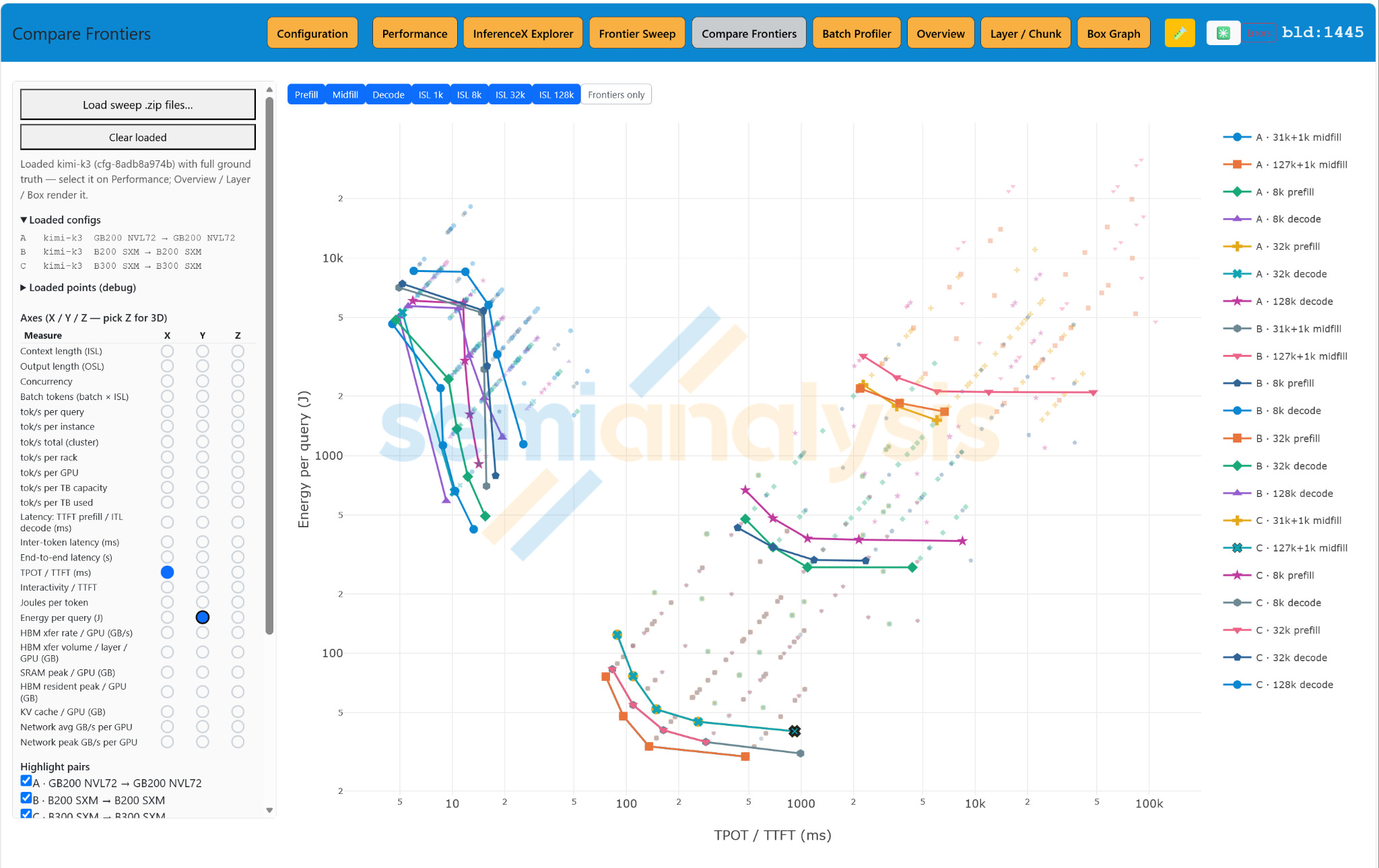
23. 示例:Kimi K3 在 Blackwell 系统上的预计性能

前面的部分描述了一种推理模型放置的方法。一个有用的检查是将其应用于特定的前沿模型,并共同探索由此产生的权衡。以下图表显示了在 B200、B300 和 GB200 系统上使用机架中 16 到 64 个 GPU 配置的 Kimi K3 建模性能。这些是工作负载和硬件的预测,而不是测量的基准测试结果。连接线标识了预计的帕累托前沿:在不放弃吞吐量或其他选定目标的情况下无法改善交互性的配置。

22.1 交互性和吞吐量

第一张图比较了 decode 的每个输出 token 时间,或 prefill 和 midfill 的首 token 时间,与每 GPU 每秒 token 数的关系。将吞吐量归一化为每 GPU 使得不同大小的配置可以直接比较。

左下组包含 8k 和 32k 输入上下文的 decode 前沿。所有三种 GPU 类型都出现了可行的配置。GB200 在前沿的大部分区域都很强,而 B200 和 B300 也提供了有竞争力的点。最低延迟的 decode 配置通常结合了流水线和张量并行。在面向吞吐量的一端,每 GPU 每秒最高 token 数通常来自每 GPU 一个 attention 实例,没有张量或流水线并行,而专家并行保持系统允许的最大宽度。

中上组是 midfill:127k 缓存输入 token,后跟 1k token 附加,然后 decode。GB200 在没有流水线并行的情况下使用 TP=4 或 TP=2 领先于低 TTFT 部分。B300 在面向吞吐量的一端赶上来。B200 和 B300 通常使用 PP=4,专家并行在每个阶段内有界,因此专家 all-to-all 保留在节点内。

右上的两组是 8k 和 32k token prefill。所有三种 GPU 类型都收敛于相似的配置:PP=4,TP=4 或 TP=2 有利于降低 TTFT,但牺牲了一些吞吐量。它们接近的预计性能反映了共享的 Blackwell 计算架构以及这些 prefill 工作负载的计算受限性质。

[

](https://substackcdn.com/image/fetch/$s_!4rOA!,f_auto,q_auto:good,fl_progressive:steep/https%3A%2F%2Fsubstack-post-media.s3.amazonaws.com%2Fpublic%2Fimages%2F3f424d0d-368f-461d-8b78-5433bed03128_2048x1274.png)图 26. decode、midfill 和 prefill 的预计交互性和吞吐量前沿。来源:SemiAnalysis Inference Simulator。

22.2 每次查询的能耗

第二张图使用相同的模拟配置,但将纵轴更改为每个已完成查询的能耗。Decode 是最大的能耗工作负载,因为建模的输出长度为 1,000 个 token,每个查询需要大约 1,000 次通过模型。Midfill 使用最少的能量:它在通过现有长上下文一次后附加一个相对较短的序列。完整的 8k 和 32k prefill 需要依次更多的能量。

该模型包括 Kimi K3 的局部注意力层,因此保留的状态和计算都反映了注意力结构带来的预期节省,而不是将每一层都视为全注意力。

[

](https://substackcdn.com/image/fetch/$s_!L_rU!,f_auto,q_auto:good,fl_progressive:steep/https%3A%2F%2Fsubstack-post-media.s3.amazonaws.com%2Fpublic%2Fimages%2F0ab3a5dc-803c-4d91-b513-ca10e9ea2df6_2048x1289.png)图 27. 相同 decode、midfill 和 prefill 前沿的预计每次查询能耗。来源:SemiAnalysis Inference Simulator。

22.3 快速内存需求

第三张图显示了每个 GPU 的峰值 HBM 驻留。它排除了 KV 状态进入或离开 worker 时使用的额外缓冲区,这可能会为每个 GPU 增加几 GB。在对话或代理轮次之间,非活动的 KV blob 可以并行传输到网络附加 DDR,包括附加到节点 CPU 的 DRAM。该内存更便宜、更可用,且较少受到 HBM 供应链的限制。

预计前沿聚集在可行内存范围的下端附近。对于 prefill 和 midfill,下降的步骤来自添加流水线并行和增加张量或数据并行,包括数据并行环形批处理实例。Decode 首先通过张量或数据并行减少每 GPU 驻留,稍后使用流水线并行。

即使考虑了实际的 KV 传输缓冲区,大多数前沿配置仍保持在每 GPU 约 80 GB 以下。这支持了早先的结论,即只要更广泛的存储和编排系统及时移动空闲状态,带宽就可能比在每个加速器上最大化 HBM 容量更有价值。

[

](https://substackcdn.com/image/fetch/$s_!-v6T!,f_auto,q_auto:good,fl_progressive:steep/https%3A%2F%2Fsubstack-post-media.s3.amazonaws.com%2Fpublic%2Fimages%2Faf12d141-27cf-4c91-9532-9978c5a3a792_2792x1796.png)图 28. 模拟前沿中每个 GPU 的预计峰值 HBM 驻留。来源:SemiAnalysis Inference Simulator。

22.4 网络峰值和纵向扩展边界

第四张图显示了每个 GPU 的预计峰值网络流量。Prefill 和 midfill 密集使用网络进行专家并行,因为许多路由激活同时在进行中。因此,流水线并行在 B200 和 B300 系统上特别有用:将一个阶段放在节点内可以将其专家 all-to-all 流量保留在本地 NVLink 网络上。

GB200 NVL72 将纵向扩展带宽延伸到整个机架。因此,更多的 GPU 可以并行参与一层,所有实例同步推进该层,从而在不跨越较弱网络边界的情况下改善延迟和吞吐量。

Decode 显示了较低的区间平均峰值,因为小批次一次只咨询相对较少的专家。单个传输仍以物理 NVLink 速率突发;绘制的较低值反映了比传输本身更长的测量间隔。瞬时链路速率和持续流量之间的这种区别在调整网络规模和解释利用率时很重要。

[

](https://substackcdn.com/image/fetch/$s_!485f!,f_auto,q_auto:good,fl_progressive:steep/https%3A%2F%2Fsubstack-post-media.s3.amazonaws.com%2Fpublic%2Fimages%2F8f02faa0-a5dd-4f3f-bc27-37c4f6912894_2652x1652.png)图 29. 每个 GPU 的预计峰值网络流量以及将专家流量保留在纵向扩展域内的好处。来源:SemiAnalysis Inference Simulator。

这四个视图讲述了一个一致的故事。最佳配置随着操作模式和延迟-吞吐量前沿上的选定点而变化。Prefill 和 midfill 奖励有组织的并行和阶段本地专家流量。Decode 在低延迟端受益于并行,但每 GPU 最高吞吐量来自更简单的 attention 实例与宽泛专家放置的结合。在预计的前沿中,快速内存容量似乎不如网络放置、内存带宽和编排具有限制性。

结语视角

推理的有用分析单位不仅仅是总参数量。它是与机器的内存、通信和时间层次结构相结合的模型活动流。

MoE 提供了结构。层组重复。专家众多但可单独管理。Attention 宽泛且越来越多地由 KV 状态塑造。操作按顺序发生并可以重用硬件。流水线、张量和专家并行都可以遵循其最自然的维度。Prefill 和 midfill 可以将路由排序为高效的专家批次,而 decode 可以保持短批次和高交互性。

硬件可以反映该结构。逻辑加速器对等集提供有限的纵向扩展域。节点堆叠成机架。机架可以是一个纵向扩展 worker 或几个流水线阶段。共享存储使 KV blob 可移动。数据中心网络连接有限的 worker,而不是承载每个内部张量操作。调度使可预测和随机阶段保持稳定流。

以这种方式把握问题并不能消除其规模。它使该规模更容易划分。模型、worker、机架、存储系统和调度器成为一个连贯设计的各个部分,可以被测量、说明和改进。

Mixture of Experts, now widely used in frontier models, has changed both the structure of serving and the economics of useful inference. It did more than increase parameter count. It changed which tensors are active for each token, what must remain close together, which transfers need strong local bandwidth, which can tolerate a weaker network link, and how memory movement, storage, and scheduling contribute to useful throughput.

混合专家模型现已广泛应用于前沿模型中,它不仅改变了服务的结构,也改变了有效推理的经济学。它的作用远不止增加参数量。它改变了每个 token 激活哪些张量,哪些数据必须保持紧密聚合,哪些传输需要强大的本地带宽,哪些可以容忍较弱的网络连接,以及内存移动、存储和调度如何为有效吞吐量做出贡献。

The best place to begin is the service as a whole. Inference runs inside a cluster coordinated by an orchestration layer such as NVIDIA Dynamo, Mooncake, or a custom scheduler. These work closely with inference servers like vLLM or SQlang, and those also have their own orchestration features. This article will not go into the details of how you work with the orchestration software or which you should choose. The article aims to provide an overview of the process and reasons for various features you may use.

最佳的切入点是整体服务。推理运行在一个由编排层(如 NVIDIA Dynamo、Mooncake 或自定义调度器)协调的集群内。这些编排层与 vLLM 或 SQlang 等推理服务器紧密协作,而这些服务器本身也具备各自的编排特性。本文不会深入探讨如何使用编排软件或该如何选择的细节。本文旨在概述您可能使用的各种特性的流程及其背后的原因。

A user (or their agent) starts a conversation with a request (query), and the conversation may continue after answers with more requests. The request- answer is a “turn”. In modern AI systems the user is often running a in a client application (whether GUI or command-line oriented) and some of the answers coming back from the AI are intercepted by that application as instructions for it to run, things like editing your code or searching your company guidelines on an HR question.

用户(或其代理)通过请求开始对话,并在收到回答后可能继续发起更多请求。这种“请求-回答”过程构成一个“轮次”。在现代 AI 系统中,用户通常在客户端应用程序(无论是 GUI 还是命令行界面)中运行,而从 AI 返回的部分回答会被该应用程序拦截作为其执行的指令,例如编辑您的代码或就人力资源问题搜索公司指南。

The AI system can also do some of those things itself from its data center, for example it may search the web. The results from these intercept tool actions are also returned to the AI as requests, creating more turns. The server keeps a context (often referred to as KV cache or just cache) which is the distillation of the session, allowing each new request, from user or from tool, to be properly interpreted for overall forward progress. There can be thousands of turns per hour when the user launches an agent on a long-running task. The conversation can also pause and resume hours or even days later.

AI 系统也可以在其数据中心内自行完成其中某些操作,例如搜索网络。这些拦截工具操作的结果也会作为请求返回给 AI,从而产生更多轮次。服务器会维护一个上下文(通常被称为 KV cache 或直接称为 cache),它是整个会话的精华,使得来自用户或工具的每个新请求都能被正确解释,以实现整体的向前推进。当用户启动代理执行长时间运行的任务时,每小时可能会产生数千个轮次。对话也可以暂停,并在几小时甚至几天后恢复。

When a request arrives at the inference servers the orchestration puts it into a queue, while will feed into an input-fill worker, along with any context from system prompts and prior turns in the conversation. The query is then converted into new context appended to the conversation. That new context state is then moved to a decode worker. Decode repeatedly reads the accumulated state, generates answer tokens, and those answer tokens are also appended to the conversation state. The process may loop through tools, agents, users, and further input-fill work. A model worker running on GPUs is only one part of this token factory; storage, networking, and orchestration connect its stages.

当请求到达推理服务器时,编排器会将其放入队列,随后将连同系统提示词和对话中先前轮次的上下文一起输入到 input-fill worker 中。然后,该查询被转换为新的上下文并附加到对话中。接着,这个新的上下文状态被移动到 decode worker。Decode worker 会反复读取累积的状态,生成回答 token,而这些回答 token 也会被附加到对话状态中。这个过程可能会在工具、代理、用户以及进一步的 input-fill 工作之间循环。在 GPU 上运行的模型 worker 只是这个 token 工厂的一部分;存储、网络和编排将它的各个阶段连接起来。

Inside the workers, four operating regimes are worth distinguishing from the beginning:

在 worker 内部,有四种操作模式从一开始就值得区分:

1.

1.

Prefill, where the initial block of new tokens is processed together.

Prefill,即初始的新 token 块被一起处理的阶段。

2.

2.

Midfill, where a continuation request is appended to an existing cached context.

Midfill,即延续请求被附加到现有缓存上下文中的阶段。

3.

3.

Decode attention, where the context is used to generate the basics of newly generated tokens.

Decode attention,即使用上下文生成新 token 基础的阶段。

4.

4.

Decode experts, where each basic new token is refined by a selection of experts a large total set of possible experts.

Decode experts,即每个基础新 token 由从大量可能的专家中选出的部分专家进行细化的阶段。

These regimes place different demands on compute, memory, and networking. Prefill and midfill are closely related, with Prefill being a Midfill with zero prior context. However, Prefill is a common special case, corresponding to one-shot queries like classic “”chatbot” use, and can be optimized a bit differently than Midfill. Prefill reaches high arithmetic intensity (ratio of computation to data movement) and does not need to wait for context to be located and read. Midfill begins from an existing KV cache for prior state and appends a new request input sequence. This generally has a more moderate arithmetic intensity than prefill because there are fewer new tokens and more existing data to move per token.

这些模式对计算、内存和网络提出了不同的要求。Prefill 和 midfill 密切相关,Prefill 可以看作是先前上下文为零的 Midfill。然而,Prefill 是一种常见的特殊情况,对应于经典的“聊天机器人”使用等一次性查询,其优化方式可能与 Midfill 略有不同。Prefill 达到了很高的算术强度(Arithmetic Intensity,即计算量与数据移动量的比率),并且不需要等待上下文定位和读取。Midfill 从用于先前状态的现有 KV cache 开始,并附加新的请求输入序列。这通常具有比 prefill 更温和的算术强度,因为每个 token 对应的新 token 更少,而需要移动的现有数据更多。

Decode attention and decode expert work are generally low arithmetic intensity since there are few new tokens compared to the prior context or expert weights, which at decode state are data that needs to be moved. Meanwhile, across all of them, the tensors for attention and for experts are the same regardless of token value, so there is benefit to sharing a single reading of a tensor with as many tokens as can be queued to use it, even tokens coming from unrelated requests by other users which simply happen to be running at the same time and which are networked closely enough to share. Treating all four mode as the same workload gives away much of the structural advantages that MoE models offer in terms of different intensity and different sharing patterns.

Decode attention 和 decode expert 工作通常具有较低的算术强度,因为与先前上下文或专家权重相比,新 token 很少,而在 decode 状态下这些权重是需要移动的数据。同时,在所有模式中,无论 token 的值如何,attention 和 expert 的张量都是相同的,因此,将一次张量读取共享给尽可能多的可排队使用的 token 是有益的,甚至是那些恰好同时运行且网络距离足够近以实现共享的、来自其他用户不相关请求的 token。将这四种模式视为相同的工作负载,会丧失 MoE 模型在 不同强度和不同共享模式方面所提供的许多结构优势。

In this document we will treat the 4 stages separately, and sometimes assume they are disaggregated. There are tradeoffs between aggregated (where the models stay on one server, which reconfigures as the request progresses between the stages) and disaggregated where the orchestrator may find a free slot on another machine already configured appropriately. Generally we will talk about the stages as disaggregated, with aggregation being a special case of always making the current node available when a previous stage finishes. There will be a section on the trade-offs at the end, after the work to be done has been more completely introduced.

在本文中,我们将分别讨论这 4 个阶段,有时会假设它们是分离的。在聚合(模型保留在一个服务器上,随着请求在各个阶段之间推进而重新配置)和分离(编排器可以在另一台已经适当配置的机器上找到空闲槽位)之间存在权衡。通常,我们将这些阶段作为分离状态来讨论,而聚合则是“当前一阶段完成时始终使当前节点可用”的一种特例。在更全面地介绍要完成的工作之后,文末将有一节专门讨论这些权衡。

A transformer model is a deep stack of repeating layer groups. A group may contain one kind of layer, or it may contain a full-attention layer together with several linear, local, selective, or otherwise optimized-attention layers (this is a hybrid group of layers). Within each layer, attention, shared transformations, routing, selected experts, and recombination occur in sequence. Those steps are known in advance and repeat continuously, allowing the same hardware resources to serve different parts of the flow at different moments.

Transformer 模型是一个由重复层组构成的深层堆栈。一个组可能包含一种类型的层,也可能包含一个全注意力层以及多个线性、局部、选择性或其他优化注意力层(这是一个混合层组)。在每一层内,注意力、共享变换、路由、选定的专家和重组按顺序发生。这些步骤是预先知晓并不断重复的,允许相同的硬件资源在不同时刻服务于流程的不同部分。

The machines can also be described equally simple recurring units. A node is a group of accelerators, typically a tray in a rack, each accelerator pairs compute with local fast memory. A node is coordinated by a CPU and connected to other nodes through NICs (network interface controller). Nodes stack into racks. A rack may act as one scale-up domain when very large tensors are , several smaller scale-up islands, or a set of pipeline stages. Datacenter networking then joins bounded workers to storage and orchestration rather than participating in every inner tensor operation.

机器也可以被描述为同样简单的重复单元。一个节点是一组加速器,通常是机架中的一个托盘,每个加速器将计算与本地快速内存配对。节点由 CPU 协调,并通过 NIC(网络接口控制器)连接到其他节点。节点堆叠成机架。当非常大的张量被处理时,机架可以作为一个纵向扩展域,或者作为几个较小的纵向扩展岛,或一组流水线阶段。然后,数据中心网络将有限的 worker 连接到存储和编排,而不是参与每一个内部张量操作。

This essay follows that progression. It begins with the global service and the operating regimes, then opens the model into wide layer-group slices and maps them onto accelerator nodes and racks. From there it develops pipeline, tensor, and expert parallelism; the limit imposed by KV-cache memory; the different value of batching in prefill, midfill, and decode; and the role of scheduling in a many-rack token factory.

本文遵循这一进展。它从全局服务和操作模式开始,然后将模型展开为宽泛的层组切片,并将它们映射到加速器节点和机架上。由此,它进一步阐述了流水线并行、张量并行和专家并行;KV cache 内存带来的限制;在 prefill、midfill 和 decode 中批处理的不同价值;以及调度在多机架 token 工厂中的作用。

[

[

](https://substackcdn.com/image/fetch/$s_!nG_t!,f_auto,q_auto:good,fl_progressive:steep/https%3A%2F%2Fsubstack-post-media.s3.amazonaws.com%2Fpublic%2Fimages%2F0e02df36-fc57-4ee4-9015-52aa09fd7c07_2500x1470.png)Figure 1. Overview of model stages in an inference service.

](https://substackcdn.com/image/fetch/$s_!nG_t!,f_auto,q_auto:good,fl_progressive:steep/https%3A%2F%2Fsubstack-post-media.s3.amazonaws.com%2Fpublic%2Fimages%2F0e02df36-fc57-4ee4-9015-52aa09fd7c07_2500x1470.png)图 1. 推理服务中模型阶段概述。

1. Orchestration delivers requests via queues into pools of workers

1. 编排通过队列将请求传递到 worker 池

An inference service is a cluster where prior requests and immutable state are stored when idle and then queued for delivery to specialized workers when a new request pulls in context or a prior request reawakens for continuation. The incoming queue is not yet a batch. Each request carries prompt tokens, references to reusable context, service objectives, and often an existing conversation or agent state. An orchestrator may place it into a prefill, midfill, or decode batch, and the request can join or leave that batch independently as it completes, making that capacity available for new work. Continuous batching works best when the scheduler knows which workers have slots that match the request’s context length and service objective.

推理服务是一个集群,在空闲时存储先前的请求和不可变状态,然后当新请求引入上下文或先前请求重新唤醒以继续时,将它们排队以交付给专门的 worker。进入队列的请求还不是批次。每个请求携带提示 token、对可重用上下文的引用、服务目标,通常还有现有的对话或代理状态。编排器可以将其放入 prefill、midfill 或 decode 批次中,并且请求可以在完成时独立加入或离开该批次,从而释放该容量用于新工作。当调度器知道哪些 worker 拥有与请求的上下文长度和服务目标相匹配的槽位时,连续批处理的效果最好。

Prefill workers create context from a substantial block of new tokens. Their output is new KV state for every model layer, stored independently of the worker that created it. The KV state moves along model layers, the output of layer K from one turn becomes input to layer K in the next turn. In pipelined servers this creates a natural “torrenting” of output and input from separate NICs.

Prefill worker 从大量新 token 块中创建上下文。它们的输出是每个模型层的新 KV 状态,独立于创建它的 worker 存储。KV 状态沿着模型层移动,上一轮中第 K 层的输出成为下一轮中第 K 层的输入。在流水线服务器中,这创造了来自不同 NIC 的输出和输入的自然“洪流”。

Midfill workers extend previously processed context. The cached prefix may contain system and user prompts, memories, earlier conversation turns, agent steps, or retrieved documents. Large roots may be already cached, while the incremental input can be much smaller than a comparable uncached request: a half-million context may receive only a few hundred or a few thousand new tokens.

Midfill worker 扩展先前处理过的上下文。缓存的前缀可能包含系统和用户提示词、记忆、较早的对话轮次、代理步骤或检索到的文档。大的根节点可能已经被缓存,而增量输入可能比未缓存的可比请求小得多:一个五十万上下文可能只接收几百或几千个新 token。

Decode workers consume the processed, accumulated context and generate one or a few tokens (multi-token prediction is becoming quite common) per pass. Every generated token adds a small amount of new state. The same context can later return to a midfill worker when a user, tool, or agent contributes another block of input. Agentic work using tools creates a repeated sequence of context extension and generation, not merely one prefill followed by one decode.

Decode worker 消耗已处理、累积的上下文,并在每次传递中生成一个或几个 token(多 token 预测正变得相当普遍)。每个生成的 token 都会添加少量新状态。当用户、工具或代理贡献另一个输入块时,相同的上下文稍后可以返回到 midfill worker。使用工具的代理工作创建了上下文扩展和生成的重复序列,而不仅仅是一个 prefill 后跟一个 decode。

A worker may occupy a node, a tray, or a rack. The service becomes large by operating many bounded workers and moving requests and state among them. Depending on precision and working-state requirements, even multi-trillion-parameter models can fit within the aggregate memory of a modern rack-scale system. The datacenter network remains essential because the factory must connect many such workers to shared storage and continuously match worker configurations to demand. KV transfers may be gigabytes in size, but they can be striped or torrented across multiple links and destinations; their movement time can remain well below the lifetime of a long decode job.

一个 worker 可能占据一个节点、一个托盘或一个机架。服务通过操作许多有限的 worker 并在它们之间移动请求和状态而变大。根据精度和工作状态要求,即使是数万亿参数的模型也可以装入现代机架级系统的聚合内存中。数据中心网络仍然必不可少,因为工厂必须将许多这样的 worker 连接到共享存储,并不断使 worker 配置与需求相匹配。KV 传输可能在千兆字节级别,但它们可以跨多个链路和目标进行条带化或洪流式传输;它们的移动时间可以远低于长时间 decode 任务的持续时间。

This separation is useful for both performance and operations. Prefill and midfill are predictable once the cached-prefix size, new-token count, and worker configuration are known. Decode completion time is stochastic because arrival of the final output token cannot be predicted in advance. Shared memory and storage between the pools let each stage run at its own cadence. Later sections of this article will discuss queues, ready buffers, and worker reconfiguration. For now, the important point is that the service is a loop of stages joined by movable state.

这种分离对性能和操作都很有用。一旦知道了缓存前缀大小、新 token 数量和 worker 配置,Prefill 和 midfill 就是可预测的。Decode 完成时间是随机的,因为无法提前预测最终输出 token 的到达时间。池之间的共享内存和存储让每个阶段能以自己的节奏运行。本文后面的部分将讨论队列、就绪缓冲区和 worker 重新配置。目前,重要的一点是,服务是一个由可移动状态连接的阶段循环。

AgentX examples

AgentX 示例

[

[

](https://substackcdn.com/image/fetch/$s_!xosE!,f_auto,q_auto:good,fl_progressive:steep/https%3A%2F%2Fsubstack-post-media.s3.amazonaws.com%2Fpublic%2Fimages%2F50dba89e-9dfd-4d9d-831c-3dcd1748a45e_2022x776.png)Figure 2. “CC Traces Weka” dataset contributed to AgentX, release 34. Source: SemiAnalysis AgentX.

](https://substackcdn.com/image/fetch/$s_!xosE!,f_auto,q_auto:good,fl_progressive:steep/https%3A%2F%2Fsubstack-post-media.s3.amazonaws.com%2Fpublic%2Fimages%2F50dba89e-9dfd-4d9d-831c-3dcd1748a45e_2022x776.png)图 2. 贡献给 AgentX 第 34 版的“CC Traces Weka”数据集。来源:SemiAnalysis AgentX。

This is viewed with the SemiAnalysis Conversation Explorer. It shows that context growth during conversations can be quite rapid but also goes through large fluctuations due to compaction and other model behavior which may not be explained in public discussions. Orchestration of the inference context is a competitive advantage for AI companies.

这可以通过 SemiAnalysis Conversation Explorer 查看。它表明对话期间的上下文增长可能非常迅速,但由于压缩和其他模型行为(这些行为可能未在公开讨论中解释)也会经历大幅波动。推理上下文的编排是 AI 公司的竞争优势。

[

[

](https://substackcdn.com/image/fetch/$s_!lXqX!,f_auto,q_auto:good,fl_progressive:steep/https%3A%2F%2Fsubstack-post-media.s3.amazonaws.com%2Fpublic%2Fimages%2Fc1a155ad-ce74-4b40-a4bc-b1e4af1fa624_1510x1230.png)Figure 3. Cache, new input, and result lengths seen at each turn of the same conversations. Source: SemiAnalysis AgentX.

](https://substackcdn.com/image/fetch/$s_!lXqX!,f_auto,q_auto:good,fl_progressive:steep/https%3A%2F%2Fsubstack-post-media.s3.amazonaws.com%2Fpublic%2Fimages%2Fc1a155ad-ce74-4b40-a4bc-b1e4af1fa624_1510x1230.png)图 3. 相同对话的每个轮次中看到的缓存、新输入和结果长度。来源:SemiAnalysis AgentX。

We can take that same dataset and pull out the cache, new input, and result length values seen at every turn. This visual shows how the Token Factory needs to serve many different workloads. In principle there could be requests similar to each dot in those traces (and more dots from other workload datasets) all running at the same time, assigned to some worker in the AI cluster.

我们可以提取相同的数据集,并提取在每个轮次中看到的缓存、新输入和结果长度值。此可视化展示了 Token 工厂需要如何服务于许多不同的工作负载。原则上,这些轨迹中的每个点(以及来自其他工作负载数据集的更多点)所代表的请求可能同时运行,并分配给 AI 集群中的某个 worker。

This article aims to survey some of the major functions in inference that make it possible,

本文旨在概述推理中使其成为可能的一些主要功能,

2. KV state moves as immutable blobs

2. KV 状态作为不可变 blob 移动

Reusable context at data-center scale becomes a shared object-store of immutable blobs rather than a file attached to one machine. A system prompt, project context, previous user turns, tool output, and generated tokens can be in separate blobs. A new operation reads the blobs it needs and appends new ones; existing blobs normally remain unchanged. This forward-only structure follows the causal transformer itself. Changes can be handled by backtracking and creating a new branch rather than rewriting the common path.

数据中心规模下的可重用上下文成为不可变 blob 的共享对象存储,而不是附加到一台机器上的文件。系统提示词、项目上下文、先前的用户轮次、工具输出和生成的 token 可以位于单独的 blob 中。一个新操作读取它需要的 blob 并附加新的 blob;现有的 blob 通常保持不变。这种仅向前的结构遵循因果 Transformer 本身。变更可以通过回溯并创建新分支来处理,而不是重写公共路径。

The durable source of these blobs is a fast, parallel, scale-out memory and storage pool. It needs enough aggregate bandwidth and network reach that prefill, midfill, and decode workers can be selected for suitability and availability rather than because one machine owns the only copy of the context. Newly idle blobs can first move into shared network-attached DRAM, including node-CPU memory and dedicated memory appliances. As that tier fills, a classifier can discard blobs that are not likely for reuse, or promote longer-lived state to SSD. The underlying text and references are often orders of magnitude smaller than the expanded KV representation, so it is possible rebuild a KV blob from that smaller text if the triage decided to reuse space and discarded the expanded embedded state. AI calculations can vary subtly, so while the rebuilt state can be expected to be a valid context, services may take different approaches to how casually they discard and rebuild, and how much they try to keep important immutable state.

这些 blob 的持久来源是一个快速、并行、横向扩展的内存和存储池。它需要足够的聚合带宽和网络覆盖范围,以便可以根据适用性和可用性来选择 prefill、midfill 和 decode worker,而不是因为某台机器拥有上下文的唯一副本。新空闲的 blob 可以首先移动到共享的网络附加 DRAM 中,包括节点 CPU 内存和专用内存设备。当该层填满时,分类器可以丢弃不太可能重用的 blob,或将寿命较长的状态提升至 SSD。底层文本和引用通常比扩展的 KV 表示小几个数量级,因此如果分类决定重用空间并丢弃了扩展的嵌入状态,则可以从较小的文本重建 KV blob。AI 计算可能会有细微差别,因此虽然可以预期重建的状态是有效的上下文,但服务在随意丢弃和重建的频率,以及努力保留重要不可变状态的程度方面,可能会采取不同的方法。

For a deeper dive on how the blobs are managed, Unified Radix Cache: One Tree for Hybrid Model Prefix Caching - LMSYS Org is recommended reading. It is not the last word, but it is clearly written and will point you to other sources if you want to look for more.

要深入了解 blob 是如何管理的,推荐阅读 Unified Radix Cache: One Tree for Hybrid Model Prefix Caching - LMSYS Org。它不是最终定论,但它写得很清晰,如果您想寻找更多信息,它会为您指引其他来源。

There are also frequent compactions of state with long-running agents that build up to the maximum context, so in general after a compaction there will be many prior blobs which have been abandoned in favor of a new context. The space from the pre-compaction contexts is probably recycled for new work.

对于累积到最大上下文的长时间运行代理,状态也会频繁压缩,因此通常在压缩后会有许多先前的 blob 被放弃,转而支持新的上下文。压缩前上下文占用的空间可能会被回收用于新工作。

[

[

](https://substackcdn.com/image/fetch/$s_!aFGC!,f_auto,q_auto:good,fl_progressive:steep/https%3A%2F%2Fsubstack-post-media.s3.amazonaws.com%2Fpublic%2Fimages%2Fa1426880-84ea-42b8-be37-ea5e967ad662_2032x816.png)Figure 4. AgentX release 34, selected conversations. Source: SemiAnalysis AgentX.

](https://substackcdn.com/image/fetch/$s_!aFGC!,f_auto,q_auto:good,fl_progressive:steep/https%3A%2F%2Fsubstack-post-media.s3.amazonaws.com%2Fpublic%2Fimages%2Fa1426880-84ea-42b8-be37-ea5e967ad662_2032x816.png)图 4. AgentX 第 34 版,选定的对话。来源:SemiAnalysis AgentX。

You can see compactions occur in the right half of these conversations as contexts get close to the practical context limit for each model (250k tokens for Opus 4.8, 1MT for Fable). There are also “stalactites” in both lines which seem transient and reflect some proprietary behavior in Anthropic models.

您可以看到在这些对话的后半部分,随着上下文接近每个模型的实际上下文限制(Opus 4.8 为 250k token,Fable 为 1MT),发生了压缩。两行中还有“钟乳石”,它们似乎是瞬态的,反映了 Anthropic 模型中的一些专有行为。

Accelerator HBM is the “hot” working tier. It is too expensive and supply-constrained to be a good default for passive context storage. The active prefix and suffix should enter HBM shortly before use and leave promptly after the worker has finished with them. CPU DRAM is a useful staging and assembly tier, especially for outgoing state: a completed worker can move newly generated blobs into CPU memory while the storage system chooses placement and redundancy, after which the NIC sends them into the shared pool.

加速器 HBM 是“热”工作层。它太贵且供应受限,不适合作为被动上下文存储的默认选择。活动的前缀和后缀应在使用前不久进入 HBM,并在 worker 完成使用后迅速离开。CPU DRAM 是一个有用的暂存和组装层,特别是对于输出状态:一个完成的 worker 可以将新生成的 blob 移动到 CPU 内存中,同时存储系统选择放置位置和冗余,之后 NIC 将它们发送到共享池中。

For incoming data, RDMA-capable systems may allow the network to place data directly into accelerator memory, avoiding a full copy through CPU DRAM. CPU memory still remains useful for metadata, coordination, partial assembly, fallback paths, replicas, and outgoing staging. When a worker uses multiple GPUs the incoming context can be striped directly to their destination memories in parallel.

对于传入数据,支持 RDMA 的系统可能允许网络将数据直接放入加速器内存中,从而避免通过 CPU DRAM 进行完整复制。CPU 内存对于元数据、协调、部分组装、回退路径、副本和输出暂存仍然有用。当 worker 使用多个 GPU 时,传入的上下文可以直接并行条带化到其目标内存。

Rack-level hot-blob caches can also be useful, whether implemented as memory/storage appliances or making use CPU memory which is assigned to the distributed storage pool. Very common objects such as system prompts are natural candidates. These caches should remain shared scale-out resources rather than private state that binds a request to one decode machine. HBM is several times more expensive and more supply-constrained than DDR. HBM’s best use is for data ina an active batch currently earning revenue.

机架级热 blob 缓存也很有用,无论是作为内存/存储设备实现,还是利用分配给分布式存储池的 CPU 内存。系统提示词等非常常见的对象是天然的候选者。这些缓存应保持为共享的横向扩展资源,而不是将请求绑定到一台 decode 机器的私有状态。HBM 比 DDR 贵几倍,且供应更受限。HBM 的最佳用途是用于当前正在产生收入的活跃批次中的数据。

[

[

](https://substackcdn.com/image/fetch/$s_!JBSP!,f_auto,q_auto:good,fl_progressive:steep/https%3A%2F%2Fsubstack-post-media.s3.amazonaws.com%2Fpublic%2Fimages%2F6e1c09c0-f0e2-403a-83fa-b089cb442e4e_903x597.png)Figure 5. KV blobs moving through storage and worker memory.

](https://substackcdn.com/image/fetch/$s_!JBSP!,f_auto,q_auto:good,fl_progressive:steep/https%3A%2F%2Fsubstack-post-media.s3.amazonaws.com%2Fpublic%2Fimages%2F6e1c09c0-f0e2-403a-83fa-b089cb442e4e_903x597.png)图 5. KV blob 通过存储和 worker 内存移动。

Data input is generally larger than output. Midfill commonly reads a large prefix and appends a meaningful but smaller suffix. Decode reads the accumulated context and appends only the state for one or a few generated tokens. The reads are repeated, the writes usually occur just once. The system design should show these differences directly with the width of each data path.

数据输入通常大于输出。Midfill 通常读取一个大的前缀并附加一个有意义但较小的后缀。Decode 读取累积的上下文,并仅附加一个或几个生成 token 的状态。读取是重复的,写入通常只发生一次。系统设计应通过每条数据路径的宽度直接显示这些差异。

3. Prefill, midfill, and decode create distinct operating regimes

3. Prefill、midfill 和 decode 创造了不同的操作模式

The global service contains several computational regimes. Their differences are more useful than the generic labels compute-bound and memory-bound, because each has a different opportunity for reuse and a different natural mapping onto hardware.

全局服务包含几种计算模式。它们之间的差异比 compute-bound(计算受限)和 memory-bound(内存受限)等通用标签更有用,因为每种模式都有不同的重用机会和不同的硬件自然映射。

3.1 Prefill

3.1 Prefill

Classic prefill begins with little or no reusable KV state and processes a substantial block of new tokens. Those tokens share weight loads, use matrix operations efficiently, and create enough routed activations to form useful shared-expert batches. Attention and dense transforms can reach high arithmetic intensity, so prefill is often constrained primarily by compute. Long initial input contexts can raise memory traffic but these rarely get to 100,000 tokens in length, while midfill is commonly beyond that.

经典的 prefill 几乎没有或完全没有可重用的 KV 状态,并处理一个大量的新 token 块。这些 token 共享权重加载,高效使用矩阵操作,并创建足够的路由激活以形成有用的共享专家批次。Attention 和密集变换可以达到很高的算术强度,因此 prefill 通常主要受计算限制。长的初始输入上下文会增加内存流量,但这些上下文的长度很少达到 100,000 个 token,而 midfill 通常超过这个数字。

3.2 Midfill

3.2 Midfill

Midfill appends new tokens to a much longer cached prefix. The new block can still provide hundreds or thousands of activations for shared weight and expert reuse, raising arithmetic intensity to thousands of ops per byte of data. Attention must also read a large existing KV state, which can be tens of GB. It therefore sits in a mixed regime: more arithmetic reuse than decode, but much more cached-state traffic than an initial prefill of the same new-token count.

Midfill 将新 token 附加到长得多的缓存前缀中。新块仍然可以为共享权重和专家重用提供数百或数千个激活,将算术强度提高到每字节数据数千次操作。Attention 还必须读取大量现有的 KV 状态,这可能达到几十 GB。因此,它处于一种混合模式:比 decode 有更多的算术重用,但与具有相同新 token 数量的初始 prefill 相比,其缓存状态流量要大得多。

3.3 Decode attention

3.3 Decode attention

Decode advances on input of one or a few tokens per query. Each query brings its own KV state which is similar in length to what midfill processes. While prefill differs from midfill on length of cache, decode differs from midfill in input sequence length. These one to few input tokens keep arithmetic intensity low, this work is clearly dominated by the memory movement around the KV cache.

Decode 在每个查询输入一个或几个 token 时推进。每个查询带来自己的 KV 状态,其长度与 midfill 处理的长度相似。Prefill 与 midfill 在缓存长度上有所不同,而 decode 与 midfill 在输入序列长度上有所不同。这少至一两个的输入 token 保持了较低的算术强度,这项工作显然由围绕 KV cache 的内存移动所主导。

For long contexts, the attention read can exceed the size of tensor operations associated with model weights. Attention is therefore one of the largest operations in modern decode even though most model parameters reside in experts. Delta, top-k, or linear-attention algorithm layers can reduce the burden, but periodic use of a layer with full attention remains a major memory load. Each query brings its own context, so batching queries does not change the arithmetic intensity of attention.

对于长上下文,attention 读取可能超过与模型权重相关的张量操作的大小。因此,尽管大多数模型参数位于专家中,但 attention 仍是现代 decode 中最大的操作之一。Delta、top-k 或线性注意力算法层可以减轻负担,但定期使用具有全注意力的层仍然是一个主要的内存负载。每个查询都带来自己的上下文,因此批处理查询不会改变 attention 的算术强度。

3.4 Decode experts

3.4 Decode experts

Experts are not specific to the decode phase. Everywhere the model runs the experts run, and they require no context other than one token’s embedding. The history of the query has already been compressed into the activation presented to the expert. This allows various designs that share the experts across all available GPUs, reducing memory size per GPU and increasing the memory bandwidth / memory size, or memory intensity ratio. You can look at the interval needed for a GPU to read all its experts as the best case interactivity (token rate seen by each user) and so if the memory bandwidth remains constant but the GPU is responsible for fewer experts, interactivity can be higher. The gotcha is that networking needs also rise, and the all-to-all pattern needed for routing to experts is a difficult one.

专家并非 decode 阶段特有。模型运行的地方就有专家运行,并且它们除了一个 token 的嵌入之外不需要任何上下文。查询的历史已经被压缩到呈现给专家的激活中。这允许各种设计在所有可用的 GPU 之间共享专家,从而减少每个 GPU 的内存大小,并提高内存带宽/内存大小,即内存强度比率。您可以将 GPU 读取其所有专家所需的时间间隔视为最佳情况下的交互性(每个用户看到的 token 速率),因此如果内存带宽保持不变,但 GPU 负责的专家更少,交互性就可以更高。陷阱在于网络需求也会上升,并且路由到专家所需的 all-to-all 模式是一个困难的模式。

At the end of attention (in prefill, midfill, or decode) a router calculation (a small tensor operating on the unrefined token) selects a few experts for each new token. Tokens that select the same expert can share a tensor-weight load even when they come from different requests, so long as they can be gathered together in time to take advantage of the same weight loading. In practice their may be 15,000 experts across all the layers, so taking advantage of such coincidences requires deliberate synchronization like awaiting until all queries in a batch have completed attention until switching over to sending them for expert work, and that in turn may be improved by having multiple instances in different nearby machines also synchronized to that schedule. If you have ever wondered why Nvidia makes such an effort to connect 72 GPUs so closely, this is a big part of why. In a large token factory it is feasible to have those 72 machines all running in sync, allowing the experts in one layer to be divided up to 72 ways. If a layer of the model has 256 experts then each GPU is handling only 3 or 4 in each layer, permitting very fast complete cycling through all the experts. And a lot of all-to-all traffic.

在 attention 结束时(在 prefill、midfill 或 decode 中),路由器计算(对未细化的 token 进行操作的小张量)为每个新 token 选择几个专家。选择相同专家的 token 可以共享张量权重加载,即使它们来自不同的请求,只要它们能及时聚集以利用相同的权重加载。实际上,所有层中可能有 15,000 个专家,因此利用这种巧合需要刻意的同步,例如等待批次中的所有查询完成 attention,然后再切换到发送它们进行专家工作,而这反过来可以通过让不同附近机器中的多个实例也同步到该时间表来改进。如果您曾想知道为什么 Nvidia 如此努力地将 72 个 GPU 紧密连接,这就是很大一部分原因。在一个大型 token 工厂中,让这 72 台机器全部同步运行是可行的,这允许一层的专家被分成多达 72 路。如果模型的一层有 256 个专家,那么每个 GPU 在每一层只处理 3 或 4 个专家,从而允许非常快速地完整循环所有专家。以及大量的 all-to-all 流量。

Something interesting happens if your experts can all be kept in SRAM. You need a huge number of accelerators and a monster network to collect them all to all back to the GPUs, but now there is little reason to wait for a batch to form. Each expert can run whenever it has input. The energy per byte loaded is as much as 100x better than loading from HBM, so a single token running can be as efficient as perhaps a queue of 100 was before. In return for this DAF (disaggregated attention-FFN, where the experts are the FFN) you can free up the instances from needing to be synchronized. This advantage does not help as much with prefill or midfill since they trivially have a batch of tokens they can sort into shared queues on one layer, but it still may offload all the expert weights from those GPUs allowing them to optimize their local memory for other uses like longer contexts. The networking is still a gotcha, where an SRAM based accelerator could turn around an expert calculation in less than a microsecond but now you may be flooding a switch connected to hundreds of nodes with the all to all traffic for millions of tokens. The network may absorb more money and power than the experts they connect.

如果您的专家都能保存在 SRAM 中,就会发生一些有趣的事情。您需要大量的加速器和一个庞大的网络来将它们全部 all-to-all 收集回 GPU,但现在几乎没有理由等待批次形成。每个专家只要有输入就可以运行。每加载一字节的能量消耗比从 HBM 加载好多达 100 倍,因此运行单个 token 的效率可能与以前大约 100 个队列一样高。作为这种 DAF(disaggregated attention-FFN,其中专家就是 FFN)的回报,您可以释放实例,使其无需同步。这种优势对 prefill 或 midfill 的帮助不大,因为它们轻易地拥有一批 token,可以将它们排序到一层的共享队列中,但它仍然可以卸载这些 GPU 上的所有专家权重,允许它们为其他用途(如更长的上下文)优化本地内存。网络仍然是一个陷阱,基于 SRAM 的加速器可以在不到一微秒的时间内完成专家计算,但现在您可能会用数百万个 token 的 all-to-all 流量淹没连接到数百个节点的交换机。网络吸收的资金和功率可能比它们连接的专家还要多。

[

[

](https://substackcdn.com/image/fetch/$s_!0swW!,f_auto,q_auto:good,fl_progressive:steep/https%3A%2F%2Fsubstack-post-media.s3.amazonaws.com%2Fpublic%2Fimages%2F132a56e8-d9e0-42cd-bcda-5051cab4b9b3_875x425.png)Figure 6. Prefill and midfill are separated from the closely coupled decode loop at the KV-cache boundary.

](https://substackcdn.com/image/fetch/$s_!0swW!,f_auto,q_auto:good,fl_progressive:steep/https%3A%2F%2Fsubstack-post-media.s3.amazonaws.com%2Fpublic%2Fimages%2F132a56e8-d9e0-42cd-bcda-5051cab4b9b3_875x425.png)图 6. Prefill 和 midfill 在 KV cache 边界处与紧密耦合的 decode 循环分离。

Inference workers can improve sharing by coordinating many attention instances on the same model layer. Their routed activations then draw from one layer’s expert bank, reducing the number of different experts each destination must load. In a pipelined server this also means the networking connections used for expert parallel can be local to that stage of the machine, there will never be a routing that needs experts from another layer. Even so, each decode request contributes only one new token with typically 8 to 16 routed experts per pass, and a layer may contain hundreds of experts. At small batches, sharing remains limited and memory bandwidth continues to dominate both the KV scan and the active expert loads, with very little computation per byte of weight loaded. Expert memory needs to be very low energy per bit, no matter what kind of memory is in use.

推理 worker 可以通过协调同一模型层上的许多 attention 实例来改善共享。然后,它们路由的激活从一个层的专家库中提取,减少了每个目的地必须加载的不同专家的数量。在流水线服务器中,这也意味着用于专家并行的网络连接可以是机器该阶段的本地连接,永远不需要来自另一层的专家的路由。即便如此,每个 decode 请求每次传递只贡献一个新 token,通常每个传递有 8 到 16 个路由专家,而一层可能包含数百个专家。在小批次下,共享仍然有限,内存带宽继续主导 KV 扫描和活动专家加载,每加载一字节权重的计算量非常少。无论使用何种内存,专家内存都需要具有极低的每比特能耗。

These regimes explain why prefill, midfill, and decode may prefer different worker configurations; why decode attention and decode experts can prefer different placements within a node; and why batching helps each stage by a different amount. As prefill in modern agent work rapidly expands to the 500k token range there is a lot of memory movement, especially in token decode - the stage where the model is generating useful intermediate and final results. Fast and large 3D RAM will be decisive in efficiency. Fast memory is also useful for midfill. However, capacity needs to reach a minimum level for the large contexts we now see as normal. If memory capacity is too small then the losses in networking and excessive swarms of chips can waste power compared to future memory types which will use 3D capacity expansion without giving up on throughput.

这些模式解释了为什么 prefill、midfill 和 decode 可能偏好不同的 worker 配置;为什么 decode attention 和 decode experts 可能偏好节点内的不同放置;以及为什么批处理对每个阶段的帮助程度不同。随着现代代理工作中的 prefill 迅速扩展到 500k token 范围,存在大量的内存移动,特别是在 token decode 阶段——即模型生成有用的中间和最终结果的阶段。快速且大容量的 3D RAM 在效率方面将具有决定性作用。快速内存对 midfill 也很有用。然而,对于我们现在视为正常的大上下文,容量需要达到最低水平。如果内存容量太小,那么与未来将使用 3D 容量扩展而不牺牲吞吐量的内存类型相比,网络损耗和过多的芯片集群可能会浪费功耗。

[

[

](https://substackcdn.com/image/fetch/$s_!zjGq!,f_auto,q_auto:good,fl_progressive:steep/https%3A%2F%2Fsubstack-post-media.s3.amazonaws.com%2Fpublic%2Fimages%2Fa138a4da-0245-453d-8d93-dbeca158f2f6_1171x592.png)Figure 7. Projected effect of faster memory (hybrid-bonded DRAM, super-fast 3D RAM)) on midfill and decode with 500k token context cache length. Source: SemiAnalysis model simulator with projected accelerator and GPU performance.

](https://substackcdn.com/image/fetch/$s_!zjGq!,f_auto,q_auto:good,fl_progressive:steep/https%3A%2F%2Fsubstack-post-media.s3.amazonaws.com%2Fpublic%2Fimages%2Fa138a4da-0245-453d-8d93-dbeca158f2f6_1171x592.png)图 7. 更快内存(混合键合 DRAM、超快 3D RAM)对具有 500k token 上下文缓存长度的 midfill 和 decode 的预计影响。来源:SemiAnalysis 模型模拟器,包含预计的加速器和 GPU 性能。

While Vera Rubin 72 can crush at the mid-fill layer, which is arithmetic intense, it is not so effective at the switch to memory intensive decode where the Rubin cannot fully exercise its computational prowess. With the large context there is a premium on keeping the decode work in the same node and the midfill, avoiding sending the context across the network to a different node. This could favor an all-around chip which both has super memory thruput and really efficient computation.

虽然 Vera Rubin 72 可以在算术密集的 midfill 层大显身手,但在切换到内存密集型的 decode 时,它的效果就不那么好了,因为 Rubin 无法充分发挥其计算能力。对于大上下文,将 decode 工作保持在同一节点和 midfill 中,避免跨网络将上下文发送到不同节点,具有很高的价值。这可能有利于一种全能芯片,它既具有超级内存吞吐量,又具有真正高效的计算能力。

4. Flow through an MoE prefill layer

4. 流经 MoE prefill 层

Classic prefill begins with attention. A block of new query tokens attends to reusable prefixes like the system prompt and to earlier positions in the new block. The attention operation produces one activation for every new token, and shared transformations prepare those activations for the routed-expert stage.

经典的 prefill 从 attention 开始。一个新的查询 token 块关注可重用的前缀(如系统提示词)以及新块中的较早位置。attention 操作为每个新 token 产生一个激活,共享变换为路由专家阶段准备这些激活。

The router assigns several experts to every token. If the model selects eight routed experts, each incoming token produces roughly eight routes across a bank that may contain 256 experts or more. In token order, those records are sparse and interleaved: neighboring tokens can have completely different destinations. Across the full input block, however, every expert can accumulate a short list of assigned tokens.

路由器为每个 token 分配几个专家。如果模型选择八个路由专家,每个传入 token 大约产生八条路由,跨越一个可能包含 256 个或更多专家的库。在 token 顺序中,这些记录是稀疏且交错的:相邻的 token 可能有完全不同的目的地。然而,在整个输入块中,每个专家都可以积累一个分配给它的 token 的短列表。

The worker sorts or queues the route records by expert identifier. All activations assigned to expert 037 become one message stream; those assigned to 142 become another. A single expert-weight load can then serve all activations in that bucket. Several requests can contribute to the same buckets, and separate attention instances running the same layer can merge their routed work at the expert destination. Converting token order into expert order is one of the central efficiencies of MoE prefill. Scale-up networks like NVLink can be organized as memory mapped connections so sending requests to specific experts could be mapped to pushing the message into a specific memory mapped location which is configured as a hardware queue. There is very little start and stop time. The experts can listen with the equivalent of an RDMA CIQ that again leverages hardware acceleration to deliver the message stream without need for complex protocol start and stop. Simple headers inline on the message identify the sender and receiver. A similar connection can be set up for the return flow from expert back to the decode worker.

worker 按专家标识符对路由记录进行排序或排队。所有分配给专家 037 的激活成为一个消息流;分配给 142 的成为另一个。然后,单个专家权重加载可以服务于该桶中的所有激活。多个请求可以贡献给相同的桶,并且运行同一层的独立 attention 实例可以在专家目的地合并它们路由的工作。将 token 顺序转换为专家顺序是 MoE prefill 的核心效率之一。像 NVLink 这样的纵向扩展网络可以组织为内存映射连接,因此向特定专家发送请求可以映射为将消息推入配置为硬件队列的特定内存映射位置。几乎没有启动和停止时间。专家可以使用相当于 RDMA CIQ 的方式进行监听,这再次利用硬件加速来交付消息流,而无需复杂的协议启动和停止。消息上的内联简单标头标识发送者和接收者。可以为从专家返回到 decode worker 的回流设置类似的连接。

The expert outputs are returned to token order, weighted, combined, and passed to the next layer. At the same time, attention creates new K and V state for the appended tokens. Across the model, those values form an immutable KV suffix which are used to decode the next token, and which are eventually stored as the next blob in the context for use by the next turn in the conversation.

专家输出返回到 token 顺序,进行加权、组合,并传递到下一层。同时,attention 为附加的 token 创建新的 K 和 V 状态。在整个模型中,这些值形成一个不可变的 KV 后缀,用于解码下一个 token,并最终作为下一个 blob 存储在上下文中,供对话的下一轮使用。

Prefill therefore combines two forms of weight reuse. Attention and dense transforms reuse weights across many tokens, while routed experts reuse each selected expert across the tokens collected in its bucket. The gains eventually flatten as growth in activation traffic, KV traffic, and output handling take more time compared to the tensor calculations. Batching can delay time to first token, but a single request containing several thousand new tokens already provides substantial arithmetic intensity; prefill does not always need a large number of requests in each batch to run efficiently. Modern single-socket GPUs may be able to do the prefill even on a large model for a small batch in around a second.

因此,Prefill 结合了两种形式的权重重用。Attention 和密集变换在许多 token 之间重用权重,而路由专家在其桶中收集的 token 之间重用每个选定的专家。随着激活流量、KV 流量和输出处理比张量计算花费更多时间,增益最终会趋于平缓。批处理会延迟首 token 时间,但包含数千个新 token 的单个请求已经提供了可观的算术强度;prefill 并不总是需要每个批次中有大量请求才能高效运行。现代单插槽 GPU 甚至可以在大约一秒钟内对大型模型的小批次执行 prefill。

[

[

](https://substackcdn.com/image/fetch/$s_!OrHW!,f_auto,q_auto:good,fl_progressive:steep/https%3A%2F%2Fsubstack-post-media.s3.amazonaws.com%2Fpublic%2Fimages%2F8405f00c-c10b-41b8-b2f8-c3e4dfd7b136_1426x665.png)Figure 8. Flow through an MoE prefill layer.

](https://substackcdn.com/image/fetch/$s_!OrHW!,f_auto,q_auto:good,fl_progressive:steep/https%3A%2F%2Fsubstack-post-media.s3.amazonaws.com%2Fpublic%2Fimages%2F8405f00c-c10b-41b8-b2f8-c3e4dfd7b136_1426x665.png)图 8. 流经 MoE prefill 层。

5. Flow through an MoE decode layer

5. 流经 MoE decode 层

Decode begins with a much smaller amount of new work per forward pass. The current token, or a handful of speculated tokens in MTP (multi-token prediction) is the query. Attention reads the prior KV state together with the new token’s KV entry. The new entry appends to the result and is appended to the KV state for the next pass.

Decode 在每次前向传递中以少得多的新工作开始。当前 token,或 MTP(多 token 预测)中的少量推测 token 是查询。Attention 读取先前的 KV 状态以及新 token 的 KV 条目。新条目附加到结果中,并附加到下一次传递的 KV 状态中。

For agentic contexts, the prior KV state is often a heavier read burden than the attention and expert weights used by that one token. The new query and its local projection weights are comparatively compact. Attention may be partitioned across KV heads, context ranges, memory channels, or accelerator units, after which partial results are reduced to one token activation. That activation is small enough to move cheaply even though it will trigger much larger local tensor operations in the next phase.

对于代理上下文,先前的 KV 状态通常比该 token 使用的 attention 和专家权重具有更重的读取负担。新查询及其本地投影权重相对紧凑。Attention 可以跨 KV 头、上下文范围、内存通道或加速器单元进行分区,然后将部分结果归约为一个 token 激活。该激活足够小,可以低成本移动,即使它将在下一阶段触发大得多的本地张量操作。

The activation passes through shared transformations and routing. The router selects a few experts from the available bank, and only those expert tensors become active for the current token. Their outputs are weighted, combined, projected, and passed onward.

激活通过共享变换和路由。路由器从可用库中选择几个专家,并且只有那些专家张量对当前 token 变为活动状态。它们的输出被加权、组合、投影并向前传递。

At each layer, attention creates and retains that layer’s K/V entry for the new token. The activation then advances to attention in the next layer, where the same sequence repeats. By the time the final layer produces the next token, every layer has appended its small K/V update. Those updates can be assembled into a new immutable KV suffix while the token is streamed to the client or agent.

在每一层,attention 为新 token 创建并保留该层的 K/V 条目。然后激活前进到下一层的 attention,重复相同的序列。当最终层产生下一个 token 时,每一层都附加了其微小的 K/V 更新。这些更新可以组装成一个新的不可变 KV 后缀,同时 token 被流式传输到客户端或代理。

The flow therefore contains both a broad operation and a sparse operation. Attention reads widely across private query state. Experts activate a small subset of total model capacity. The hardware mapping should support both without forcing the entire layer to use one parallelism strategy.

因此,该流程既包含宽泛的操作,也包含稀疏的操作。Attention 在私有查询状态间进行广泛读取。专家激活总模型容量的一小部分。硬件映射应同时支持两者,而不应强迫整个层使用一种并行策略。

[

[

](https://substackcdn.com/image/fetch/$s_!lj9A!,f_auto,q_auto:good,fl_progressive:steep/https%3A%2F%2Fsubstack-post-media.s3.amazonaws.com%2Fpublic%2Fimages%2F2c316fba-4573-4690-b119-d8416000b55c_1621x737.png)Figure 9. Flow through one MoE decode layer.

](https://substackcdn.com/image/fetch/$s_!lj9A!,f_auto,q_auto:good,fl_progressive:steep/https%3A%2F%2Fsubstack-post-media.s3.amazonaws.com%2Fpublic%2Fimages%2F2c316fba-4573-4690-b119-d8416000b55c_1621x737.png)图 9. 流经一个 MoE decode 层。

6. Midfill is a distinct operating regime

6. Midfill 是一种独特的操作模式

Midfill combines a long, cached prefix with a block of new tokens to prepare another turn in a conversation or agentic work. Traces show the cached input to be many times larger than the incremental query, although the incremental query typically varies from 50 to 5,000 new input tokens. The presence of cached system prompts, conversation roots, memories, prior agent steps, and retrieved documents can quickly raise conversational and agentic contexts to a million limit. AgentX datasets show frontier experts are repeatedly compressing contexts to stay under a million-token limit.

Midfill 将一个长的缓存前缀与一个新 token 块结合,为对话或代理工作中的另一个轮次做准备。轨迹显示,缓存输入比增量查询大很多倍,尽管增量查询通常在 50 到 5,000 个新输入 token 之间变化。缓存系统提示词、对话根节点、记忆、先前代理步骤和检索文档的存在,可以迅速将对话和代理上下文提高到一百万的限制。AgentX 数据集显示,前沿专家正在反复压缩上下文,以保持在百万 token 限制之下。

This makes midfill neither a small prefill nor a large decode. Like decode, it must read a substantial private KV cache. Like prefill, it processes enough new tokens to reuse weights and to sort routed activations into useful expert batches. Its arithmetic intensity can be hundreds of times greater than one-token decode, yet its cached-state traffic can be tens of times larger than that of a similarly sized initial prefill.

这使得 midfill 既不是小的 prefill,也不是大的 decode。像 decode 一样,它必须读取大量的私有 KV cache。像 prefill 一样,它处理足够多的新 token 以重用权重,并将路由激活排序为有用的专家批次。其算术强度可能比单 token decode 高数百倍,但其缓存状态流量可能比同等大小的初始 prefill 大数十倍。

Modern accelerators can generally exploit the arithmetic reuse available in a block of hundreds of tokens, so the difficult balance is often between the large KV read and the burst of routed-expert traffic. That burst does not match the smooth rhythm of a decode pipeline: a midfill can occupy a stage much longer than the decode batches in neighboring stages, leaving those stages underused.

现代加速器通常可以利用数百个 token 块中的算术重用,因此困难的平衡通常在大量 KV 读取和路由专家流量的突发之间。这种突发与 decode 流水线的平稳节奏不匹配:midfill 占用一个阶段的时间可能比相邻阶段中的 decode 批次长得多,导致这些阶段未被充分利用。

The ideal parallelism can also differ. The worked example later in this essay finds midfill configurations that use different pipeline, tensor, and expert-parallel settings from decode. Reconfiguring a GPU in the middle of a live decode pipeline can be expensive or impractical. A service may therefore benefit from a dedicated pool of midfill-optimized nodes. The hardware can be identical to the decode pool while the loaded model stages, parallelism, and batch policies differ.

理想的并行也可能不同。本文后面的示例发现,midfill 配置使用了与 decode 不同的流水线、张量和专家并行设置。在活动的 decode 流水线中间重新配置 GPU 可能成本高昂或不切实际。因此,服务可以从专用的 midfill 优化节点池中受益。硬件可以与 decode 池相同,而加载的模型阶段、并行度和批处理策略则有所不同。

[

[

](https://substackcdn.com/image/fetch/$s_!9Kjl!,f_auto,q_auto:good,fl_progressive:steep/https%3A%2F%2Fsubstack-post-media.s3.amazonaws.com%2Fpublic%2Fimages%2F87a47cb2-ded5-4daa-b7e0-6eb17ce03340_3100x2012.png)Figure 10. Midfill combines the cached-state read of decode with enough new tokens to batch model and expert work.

](https://substackcdn.com/image/fetch/$s_!9Kjl!,f_auto,q_auto:good,fl_progressive:steep/https%3A%2F%2Fsubstack-post-media.s3.amazonaws.com%2Fpublic%2Fimages%2F87a47cb2-ded5-4daa-b7e0-6eb17ce03340_3100x2012.png)图 10. Midfill 将 decode 的缓存状态读取与足够的新 token 结合,以批处理模型和专家工作。

7. The model is a tall stack of repeating layer groups

7. 模型是重复层组的高堆栈

A model’s parameter count quantifies the total learned state, but serving depends on how that state is organized and used. The model is a stack of layers, and increasingly it is useful to group those layers into repeating architectural units.

模型的参数数量量化了总学习状态,但服务取决于该状态是如何组织和使用的。模型是层的堆栈,将这些层分组为重复的架构单元变得越来越有用。

In some MoE models, a layer group is the same as one layer. In others, a group contains one full-attention layer together with several linear, delta, top-k, or otherwise optimized-attention layers. Typically 1 to 3 of the initial layers may be dense or otherwise designed to get a clean start. The rest of the model will normally repeat one recurring group pattern.

在某些 MoE 模型中,一个层组与一层相同。在其他模型中,一个组包含一个全注意力层以及多个线性、delta、top-k 或其他优化注意力层。通常,初始的 1 到 3 层可能是密集的或为了获得干净的起点而设计。模型的其余部分通常会重复一个循环的组模式。

A wide, shallow crêpe is a useful representation of a layer group. The broad surface provides room for attention, shared transforms, routing, expert capacity, and residual flow. Its shallow thickness marks the group as one slice in a much taller repeated model. It also echoes the physical form of an accelerator: a very thin active layer spread across a broad package. The crêpe is a useful intuition for mapping a wide algorithmic flow onto a wide hardware surface.

一个宽而浅的可丽饼是层组的有用表示。宽阔的表面为 attention、共享变换、路由、专家容量和残差流提供了空间。其浅薄的厚度将该组标记为更高大的重复模型中的一个切片。它也呼应了加速器的物理形态:一层非常薄的活动层分布在宽阔的封装上。可丽饼是将宽泛的算法流映射到宽泛的硬件表面的有用直觉。

The repeated structure simplifies function planning. A mapping created for one group can be reused for the next. Corresponding memory regions can hold the next group’s weights. The same compute and communication plan can execute repeatedly. Uniformity matters not only for runtime efficiency but also for compiler, kernel, and operations tooling.

重复的结构简化了功能规划。为一个组创建的映射可以重用于下一个组。相应的内存区域可以保存下一个组的权重。相同的计算和通信计划可以重复执行。统一性不仅对运行时效率很重要,对编译器、内核和操作工具也很重要。

[

[

](https://substackcdn.com/image/fetch/$s_!NvYr!,f_auto,q_auto:good,fl_progressive:steep/https%3A%2F%2Fsubstack-post-media.s3.amazonaws.com%2Fpublic%2Fimages%2F0f20bc9d-d860-4e6d-8387-5e2ba79e9bf2_732x478.png)Figure 11. Layer groups repeat the same flow.

](https://substackcdn.com/image/fetch/$s_!NvYr!,f_auto,q_auto:good,fl_progressive:steep/https%3A%2F%2Fsubstack-post-media.s3.amazonaws.com%2Fpublic%2Fimages%2F0f20bc9d-d860-4e6d-8387-5e2ba79e9bf2_732x478.png)图 11. 层组重复相同的流。

During decode, one layer is active at a time for a given token. Within that layer, several operations occur sequentially. Neighboring layers may be prefetched, and different pipeline stages may process different queries simultaneously, but the logical path of one token still climbs through the stack in order.

在 decode 期间,对于给定的 token,一次只有一个层是活动的。在该层内,几个操作按顺序发生。相邻层可以被预取,不同的流水线阶段可以同时处理不同的查询,但一个 token 的逻辑路径仍然按顺序爬过堆栈。

[

[

](https://substackcdn.com/image/fetch/$s_!RRxu!,f_auto,q_auto:good,fl_progressive:steep/https%3A%2F%2Fsubstack-post-media.s3.amazonaws.com%2Fpublic%2Fimages%2F1cf97cc6-a4b5-403e-b115-97845e79b636_752x504.png)Figure 12. One layer group opened into sequential sublayers.

](https://substackcdn.com/image/fetch/$s_!RRxu!,f_auto,q_auto:good,fl_progressive:steep/https%3A%2F%2Fsubstack-post-media.s3.amazonaws.com%2Fpublic%2Fimages%2F1cf97cc6-a4b5-403e-b115-97845e79b636_752x504.png)图 12. 一个层组展开为顺序子层。

8. Parallelism should partition the narrow dataflows of the model

8. 并行应划分模型的狭窄数据流

Parallelism is not one decision. Pipeline, tensor, and expert parallelism divide different dimensions of the model and should be judged by different communication patterns.

并行不是一个决定。流水线、张量和专家并行划分模型的不同维度,应根据不同的通信模式来评判。

Pipeline parallelism follows the layer stack

流水线并行遵循层堆栈

Layers immediately suggest pipelining. The activation passed between layers is compact—often one embedded token, a small multi-token-prediction block, or brief summaries of prior hybrid group results —while the weights and KV state used inside a layer are much larger. A pipeline stage can therefore own one or more complete layer groups and pass a relatively small activation to the next stage without overpowered networking.

层立即让人联想到流水线。在层之间传递的激活是紧凑的——通常是一个嵌入的 token、一个小的多 token 预测块,或先前混合组结果的简短摘要——而层内使用的权重和 KV 状态要大得多。因此,一个流水线阶段可以拥有一个或多个完整的层组,并将相对较小的激活传递给下一个阶段,而无需强大的网络。

Pipelining divides model weights cleanly and keeps hot within-layer communication local. Its main drawback is multi-batch occupancy: a fully active pipeline has a different query or batch in every stage. Each stage therefore holds its share of the KV state for all live streams, and the memory benefit eventually stops improving as contexts grow.

流水线清晰地划分了模型权重,并将层内热点通信保持在本地。它的主要缺点是多批次占用:一个完全活动的流水线在每个阶段都有一个不同的查询或批次。因此,每个阶段都为所有活动流持有其 KV 状态份额,并且随着上下文的增长,内存收益最终会停止提升。

Tensor parallelism belongs where one operation is intrinsically broad

张量并行属于操作本质宽泛的地方

Attention may need to divide weights and KV state across several accelerators. KV heads, context ranges, or another linear dimension can be partitioned so that each accelerator processes its share before a compact reduction of the token result. Tensor parallelism can also serve unusually large dense transforms.

Attention 可能需要在几个加速器之间划分权重和 KV 状态。可以划分 KV 头、上下文范围或其他线性维度,以便每个加速器在紧凑归约 token 结果之前处理其份额。张量并行也可以服务于异常大的密集变换。

TP should not spread automatically into every tensor of the layer. A collective that is sensible for a broad attention operation may cost more than the arithmetic of a small expert tensor.

TP 不应自动扩展到层的每个张量中。对于宽泛的 attention 操作有意义的集合通信,其成本可能高于小专家张量的算术运算。

Expert parallelism follows independent expert tensors

专家并行遵循独立的专家张量

Most MoE parameter memory may reside in experts. Experts retain no query history of their own; context arrives in the activation. The expert bank can therefore be distributed widely across a peer set and shared by several worker instances.

大多数 MoE 参数内存可能位于专家中。专家不保留自己的查询历史;上下文在激活中到达。因此,专家库可以广泛分布在一个对等集中,并由多个 worker 实例共享。

Wide expert parallelism is useful because the experts are independent and numerous. The router sends compact activations to selected destinations, and those destinations return transformed activations. Expert-parallel width can remain large even if pipeline stages become smaller, allowing switch radix and local memory placement to be chosen independently.

宽泛的专家并行是有用的,因为专家是独立且众多的。路由器将紧凑的激活发送到选定的目的地,这些目的地返回变换后的激活。即使流水线阶段变得更小,专家并行的宽度也可以保持很大,从而允许独立选择交换机基数和本地内存放置。

The general rule is straightforward: use pipeline parallelism for the vertical layer sequence, tensor parallelism for large indivisible operations, and expert parallelism for the context-free routed-expert bank. A stage fits comfortably inside a scale-up domain when its available fast memory safely exceeds its local weights, live batch state, and working buffers:

一般规则很简单:对垂直层序列使用流水线并行,对大型不可分割的操作使用张量并行,对无上下文的路由专家库使用专家并行。当一个阶段的可用快速内存安全超过其本地权重、活动批次状态和工作缓冲区时,它就能舒适地适应纵向扩展域:

M_{free,node}>\frac{W}{P}+M_{batch}+M_{working}

M_{free,node}>\frac{W}{P}+M_{batch}+M_{working}

Modern GPU nodes often exceed that threshold by multiples. When they do, the demanding bandwidth, power, and latency requirements can remain inside one node while thinner pipeline activations and KV movement use scale-out links. The rest of the fast memory is probably not earning any revenue. Data sitting idle in memory is an expense, data moving to be processed is revenue.

现代 GPU 节点通常以数倍超过该阈值。当它们做到这一点时,高要求的带宽、功率和延迟需求可以保留在一个节点内,而较薄的流水线激活和 KV 移动则使用横向扩展链路。其余的快速内存可能并没有产生任何收入。闲置在内存中的数据是开销,移动以进行处理的数据是收入。

[

[

](https://substackcdn.com/image/fetch/$s_!bgFY!,f_auto,q_auto:good,fl_progressive:steep/https%3A%2F%2Fsubstack-post-media.s3.amazonaws.com%2Fpublic%2Fimages%2F092167fa-cb58-4f8e-a168-1c60bf339415_2079x1739.png)Figure 13. Pipeline, tensor, and expert parallelism follow different dimensions of a layer group.

](https://substackcdn.com/image/fetch/$s_!bgFY!,f_auto,q_auto:good,fl_progressive:steep/https%3A%2F%2Fsubstack-post-media.s3.amazonaws.com%2Fpublic%2Fimages%2F092167fa-cb58-4f8e-a168-1c60bf339415_2079x1739.png)图 13. 流水线、张量和专家并行遵循层组的不同维度。

9. A logical accelerator node

9. 逻辑加速器节点

A logical node is easier to understand as a peer set arranged in a ring than as a literal circuit-board layout. The ring contains perhaps sixteen accelerators. Each accelerator pairs a compute region with local fast memory. The units connect through a strong scale-up fabric. A CPU coordinates workload and memory management, while a NIC connects the node to rack and datacenter resources.

将逻辑节点理解为排列成环形的对等集,比将其理解为字面上的电路板布局更容易。该环包含大约十六个加速器。每个加速器将一个计算区域与本地快速内存配对。这些单元通过强大的纵向扩展网络连接。CPU 协调工作负载和内存管理,而 NIC 将节点连接到机架和数据中心资源。

The ring is just a visualization which shows the accelerators as peers, with equal standing. I am not implying the node-internal network should be a ring. It could be hub and spoke, rail, all-to-all, torus, hypercube .. whatever floats your boat, so long as it can handle the highest dataflows the rack contains with low latency and low energy per bit. I’ll just draw it as a ring for simplicity.

环形只是一种可视化,它将加速器显示为地位平等的对等方。我并不是暗示节点内部网络应该是环形。它可以是中心辐射、轨道、全互连、环面、超立方体……只要您喜欢,只要它能以低延迟和低每比特能耗处理机架中包含的最高数据流即可。为了简单起见,我将其画成环形。

This representation avoids committing too early to package placement, board routing, or switch implementation. The actual machine may use a central switch, several switches, direct links, or a hierarchical fabric. The logical requirement is a bounded peer set with predictable fast local communication.

这种表示避免了过早承诺封装放置、电路板布线或交换机实现。实际机器可能使用中央交换机、多个交换机、直接链路或分层网络。逻辑要求是一个具有可预测快速本地通信的有限对等集。

The accelerator design may vary. One version may use SRAM-heavy processing-in-memory units. Another may use hybrid-bonded DRAM, or IGZO memory cells placed on top during BEOL processing. Another may use a hybrid-bonded high-bandwidth true 3D memory. Memory capacity and bandwidth can change while this logical model remains useful.

加速器设计可能有所不同。一个版本可能使用重 SRAM 的存内计算单元。另一个可能使用混合键合 DRAM,或在 BEOL 处理期间放置在顶部的 IGZO 存储单元。另一个可能使用混合键合的高带宽真 3D 内存。内存容量和带宽可以改变,而这个逻辑模型仍然有用。

The node is the natural place to keep work that repeats at high frequency. Attention partitions exchange compact partial results. Routed expert activations travel to local destinations. Expert outputs return for recombination. Shared state and scheduling metadata remain near the CPU. The NIC carries pipeline activations, KV blobs, and work assignments beyond the node.

节点是保存高频重复工作的自然场所。Attention 分区交换紧凑的部分结果。路由专家激活传播到本地目的地。专家输出返回以进行重组。共享状态和调度元数据保留在 CPU 附近。NIC 将流水线激活、KV blob 和工作分配传递到节点之外。

A node may be smaller than a rack like we see in an SGX node with 8 GPUs, or a scale-up system may span the whole rack like we see with NVL72. The logical symbol remains valid in either case. If scale-up already covers the rack, the separate rack-backbone level disappears and the next boundary is directly to scale-out networking.

一个节点可能比机架小,就像我们在带有 8 个 GPU 的 SGX 节点中看到的那样,或者一个纵向扩展系统可能跨越整个机架,就像我们在 NVL72 中看到的那样。无论哪种情况,逻辑符号都保持有效。如果纵向扩展已经覆盖了机架,则单独的机架主干层将消失,下一个边界直接是横向扩展网络。

[

[

](https://substackcdn.com/image/fetch/$s_!5yYB!,f_auto,q_auto:good,fl_progressive:steep/https%3A%2F%2Fsubstack-post-media.s3.amazonaws.com%2Fpublic%2Fimages%2F3ff6ec22-e5fb-405a-8165-4a6b44c92198_875x604.png)Figure 14. A 16-accelerator peer set on a scale-up fabric.

](https://substackcdn.com/image/fetch/$s_!5yYB!,f_auto,q_auto:good,fl_progressive:steep/https%3A%2F%2Fsubstack-post-media.s3.amazonaws.com%2Fpublic%2Fimages%2F3ff6ec22-e5fb-405a-8165-4a6b44c92198_875x604.png)图 14. 纵向扩展网络上的 16 加速器对等集。

10. Nodes stack to make racks

10. 节点堆叠成机架

The ring becomes more expressive when tilted as broad, shallow hardware crêpe. Several units can be stacked vertically in a rack, like model layer groups stacked in model depth.

当倾斜成宽而浅的硬件可丽饼时,环形变得更具表现力。几个单元可以在机架中垂直堆叠,就像模型层组在模型深度中堆叠一样。

This repeated form makes the model-to-hardware relationship easier to see. A layer-group crêpe can be placed onto one hardware crêpe. Several layer groups can occupy one node if memory permits. One layer group can span several tightly connected nodes if attention or expert capacity requires it. The mapping can expand or contract without changing the basic visual vocabulary.

这种重复的形式使模型与硬件的关系更容易看清。一个层组可丽饼可以放置在一个硬件可丽饼上。如果内存允许,多个层组可以占据一个节点。如果 attention 或专家容量需要,一个层组可以跨越多个紧密连接的节点。映射可以扩展或收缩,而无需改变基本的视觉词汇。

A rack may be organized in several ways:

机架可以通过几种方式组织:

-

-

one rack-wide scale-up domain;

一个机架范围的纵向扩展域;

-

-

several node-scale islands connected by a rack backbone;

由机架主干连接的多个节点级岛屿;

-

-

pipeline stages distributed among those islands;

分布在这些岛屿中的流水线阶段;

-

-

wide expert placement within each stage;

每个阶段内宽泛的专家放置;

-

-

or a mixture of stage-local scale-up and shared scale-out links.

或阶段本地纵向扩展和共享横向扩展链路的混合。

The rack backbone is therefore an optional middle level. Some systems extend the scaleup fabric across the rack needing no separate node connector. Others use strong local node fabrics and a distinct top-of-rack or shared-rail network. Above the rack, scale-out networking connects storage, prefill pools, decode pools, and other racks.

因此,机架主干是一个可选的中间层。一些系统将纵向扩展网络延伸到整个机架,不需要单独的节点连接器。其他系统使用强大的本地节点网络和独特的机架顶部或共享轨道网络。在机架之上,横向扩展网络连接存储、prefill 池、decode 池和其他机架。

The repeated rack units also help separate two kinds of scale. The model can fit within one bounded rack worker, while the factory scales by adding many workers. The first problem is function placement. The second is worker orchestration.

重复的机架单元也有助于分离两种规模。模型可以装入一个有限的机架 worker 中,而工厂通过添加多个 worker 来扩展。第一个问题是功能放置。第二个是 worker 编排。

[

[

](https://substackcdn.com/image/fetch/$s_!9JtJ!,f_auto,q_auto:good,fl_progressive:steep/https%3A%2F%2Fsubstack-post-media.s3.amazonaws.com%2Fpublic%2Fimages%2F69500e04-c899-42bb-afd9-854d41716196_2614x1376.png)Figure 15. Accelerator nodes stacked into a rack.

](https://substackcdn.com/image/fetch/$s_!9JtJ!,f_auto,q_auto:good,fl_progressive:steep/https%3A%2F%2Fsubstack-post-media.s3.amazonaws.com%2Fpublic%2Fimages%2F69500e04-c899-42bb-afd9-854d41716196_2614x1376.png)图 15. 堆叠成机架的加速器节点。

11. One layer group reuses the node over time

11. 一个层组随时间重用节点

A layer group does not require every operation in the algorithm at peak intensity simultaneously. Its operations form a repeating sequence that reuses the same hardware for different work over the decode cycle.

一个层组不需要算法中的每个操作同时达到峰值强度。它的操作形成一个重复序列,在 decode 周期内为不同的工作重用相同的硬件。

Attention may spread across much of the ring, using many memory channels and several compute units. The query and output transformations use model weights in more compact operations. Shared feed-forward work may use a dense region. Selected experts then activate local memory-and-compute regions around the ring. Recombination returns a compact result.

Attention 可能分布在环的大部分区域,使用许多内存通道和几个计算单元。查询和输出变换在更紧凑的操作中使用模型权重。共享的前馈工作可能使用密集区域。然后,选定的专家激活环周围的本地内存和计算区域。重组返回一个紧凑的结果。

The same physical accelerators can participate differently at each step. Execution units that calculate attention may later execute one or more experts. Memory channels used to stream KV state can later feed expert weights. Buffers and local links are reused as the token advances.

相同的物理加速器可以在每个步骤中以不同方式参与。计算 attention 的执行单元稍后可以执行一个或多个专家。用于流式传输 KV 状态的内存通道稍后可以提供专家权重。随着 token 的推进,缓冲区和本地链路被重用。

This time-sharing is central to an efficient design. Static diagrams can make the machine appear underused because not every block is active at once. In reality the hardware is serving a sequence of different operations, and the goal is to keep the sequence moving with little setup or synchronization overhead.

这种时分复用是高效设计的核心。静态图可能使机器看起来未被充分利用,因为并非每个块都同时处于活动状态。实际上,硬件正在服务于一系列不同的操作,目标是让序列保持移动,而几乎没有设置或同步开销。

The broad layer-group crêpe and the accelerator peer set are complementary. The crêpe shows the algorithmic flow; the ring shows the reusable physical resources beneath it. Mapping is the act of aligning each stage of the flow with a suitable subset of the ring.

宽泛的层组可丽饼和加速器对等集是互补的。可丽饼展示了算法流;环形展示了其下可重用的物理资源。映射是将流的每个阶段与环的合适子集对齐的行为。

[

[

](https://substackcdn.com/image/fetch/$s_!NjGC!,f_auto,q_auto:good,fl_progressive:steep/https%3A%2F%2Fsubstack-post-media.s3.amazonaws.com%2Fpublic%2Fimages%2F20777839-1d23-4fd0-8474-75f9dd6c7835_821x325.png)Figure 16. One layer group reuses the peer set over time.

](https://substackcdn.com/image/fetch/$s_!NjGC!,f_auto,q_auto:good,fl_progressive:steep/https%3A%2F%2Fsubstack-post-media.s3.amazonaws.com%2Fpublic%2Fimages%2F20777839-1d23-4fd0-8474-75f9dd6c7835_821x325.png)图 16. 一个层组随时间重用对等集。

12. Put throughput boundaries where the flow is smallest

12. 将吞吐量边界放在流量最小的地方

Once the model and machine are drawn as connected flows, the placement rule becomes clear: frequent, latency-sensitive communication should remain inside the strongest local fabric, while weaker links should carry compact or amortized transfers.

一旦模型和机器被绘制为连接的流,放置规则就变得清晰:频繁的、延迟敏感的通信应保留在最强的本地网络内,而较弱的链路应承载紧凑或摊销的传输。

[

[

](https://substackcdn.com/image/fetch/$s_!3hdE!,f_auto,q_auto:good,fl_progressive:steep/https%3A%2F%2Fsubstack-post-media.s3.amazonaws.com%2Fpublic%2Fimages%2Ffaccb4c8-8dad-4d10-b414-ac79c068e9bd_800x944.gif)Figure 17. The general flow of operation of an MoE pipeline stage (animated).

](https://substackcdn.com/image/fetch/$s_!3hdE!,f_auto,q_auto:good,fl_progressive:steep/https%3A%2F%2Fsubstack-post-media.s3.amazonaws.com%2Fpublic%2Fimages%2Ffaccb4c8-8dad-4d10-b414-ac79c068e9bd_800x944.gif)图 17. MoE 流水线阶段的一般操作流(动画)。

Attention partitions may exchange partial results every layer. Expert routing sends activations to selected experts and returns their outputs. This traffic is not always the largest by byte count, but it is frequent, bursty, and sensitive to synchronization. It belongs inside the chosen scale-up domain whenever practical.

Attention 分区可能每层交换部分结果。专家路由将激活发送到选定的专家并返回其输出。这种流量并不总是按字节数计算最大的,但它是频繁的、突发的,并且对同步敏感。只要可行,它应属于选定的纵向扩展域。

The activation passed between layers or layer groups is much smaller. A pipeline boundary can therefore cross a weaker link without moving the layer’s full internal working set. KV blobs are larger, but they move at worker boundaries and are amortized across many generated tokens. Their path can use striped or torrented scale-out networking and shared storage rather than consuming the innermost tensor fabric.

在层或层组之间传递的激活要小得多。因此,流水线边界可以跨越较弱的链路,而无需移动该层的完整内部工作集。KV blob 较大,但它们在 worker 边界移动,并跨多个生成的 token 进行摊销。它们的路径可以使用条带化或洪流式的横向扩展网络和共享存储,而不是消耗最核心的张量网络。

The router-to-expert boundary is typically a medium-throughput all-to-all carrying compact activations. Its difficulty often comes from endpoint count, synchronization, and routing efficiency rather than raw byte volume. Keeping it within the scale-up domain of a node or rack limits both latency and operational complexity.

路由器到专家的边界通常是承载紧凑激活的中等吞吐量全互连。其困难通常来自端点数量、同步和路由效率,而不是原始字节量。将其保持在节点或机架的纵向扩展域内可以限制延迟和操作复杂性。

This hierarchy is easier and cheaper to build than a machine in which every link is equally strong. Scale-up paths surround the operations that exchange embeddings and partial results within every layer. Scale-out links carry pipeline activations, KV movement, scheduling traffic, and traffic between bounded workers.

这种层次结构比每条链路都同样强大的机器更容易构建且成本更低。纵向扩展路径围绕着在每一层内交换嵌入和部分结果的操作。横向扩展链路承载流水线激活、KV 移动、调度流量以及有限 worker 之间的流量。

The tiers also have different latency requirements. A pipeline transfer between layer groups may barely notice a few microseconds if throughput is sufficient. By contrast, when an expert load and multiply take only a few microseconds, an additional 100 ns at each routing hop is material. The closest links should therefore be integrated tightly with the accelerator fabric, while less frequent transfers can tolerate the scale-out network.

这些层也有不同的延迟要求。层组之间的流水线传输如果吞吐量足够,可能几乎不会注意到几微秒的延迟。相比之下,当专家加载和乘法只需几微秒时,每个路由跳数增加 100 ns 就很重要。因此,最近的链路应与加速器网络紧密集成,而不太频繁的传输可以容忍横向扩展网络。

13. Pipeline by layer group where practical

13. 在可行的情况下按层组进行流水线

The layer group is the natural first candidate for pipeline placement. In a classic MoE model the group repeats one kind of layer. In newer structures it may contain one full-attention layer followed by several optimized- or localized-attention layers.

层组是流水线放置的自然首选。在经典的 MoE 模型中,该组重复一种类型的层。在较新的结构中,它可能包含一个全注意力层,后跟几个优化或局部注意力层。

Keeping a group together can preserve internal dependencies and allow one placement and compilation plan to repeat across stages. Uniform plans reduce tooling cost and simplify deployment. Kernels, memory layouts, communication schedules, monitoring, and failure recovery all become easier when each stage runs the same recurring structure.

将一个组保持在一起可以保留内部依赖关系,并允许一个放置和编译计划跨阶段重复。统一的计划降低了工具成本并简化了部署。当每个阶段运行相同的循环结构时,内核、内存布局、通信计划、监控和故障恢复都变得更容易。

It is still possible to cut a pipeline in the middle of a group, although the resulting placement is more complex. If the layers have no special cross-layer dependency, the compact activation boundary remains a low-volume link suitable for networking. A stage may contain several whole groups, one group, or part of a large group depending on memory and throughput requirements.

仍然可以在一个组的中间切断流水线,尽管由此产生的放置更为复杂。如果层没有特殊的跨层依赖,则紧凑的激活边界仍然是适合网络的低容量链路。一个阶段可以包含多个整个组、一个组或大组的一部分,具体取决于内存和吞吐量要求。

The guiding principle is not an absolute prohibition on splitting groups. It is to prefer regular boundaries and to understand when a nonuniform split is worthwhile. Tooling and operational simplicity can be as important as a small theoretical placement gain.

指导原则并不是绝对禁止拆分组。而是优先考虑规则的边界,并理解何时非均匀拆分是值得的。工具和操作的简单性与理论上的微小放置增益一样重要。

[

[

](https://substackcdn.com/image/fetch/$s_!jQh6!,f_auto,q_auto:good,fl_progressive:steep/https%3A%2F%2Fsubstack-post-media.s3.amazonaws.com%2Fpublic%2Fimages%2F1a4e2dcc-aaaf-4577-9cc4-15ea1fecab2c_683x371.png)Figure 18. Four uniform pipeline stages.

](https://substackcdn.com/image/fetch/$s_!jQh6!,f_auto,q_auto:good,fl_progressive:steep/https%3A%2F%2Fsubstack-post-media.s3.amazonaws.com%2Fpublic%2Fimages%2F1a4e2dcc-aaaf-4577-9cc4-15ea1fecab2c_683x371.png)图 18. 四个统一的流水线阶段。

14. Pipeline depth ends at the KV-cache crossover

14. 流水线深度在 KV cache 交叉点处终止

Pipeline parallelism divides model weights cleanly. If a model has weight footprint (W) and uses (P) stages, the idealized weight footprint per stage approaches (W/P).

流水线并行清晰地划分了模型权重。如果一个模型有权重占用空间 (W) 并使用 (P) 个阶段,则每个阶段的理想权重占用空间接近 (W/P)。

KV-cache demand behaves differently. A full pipeline remains occupied by running a different query or batch in every stage. In an eight-stage pipeline, each stage owns one eighth of the layer-wise KV values for each of eight live streams. The reduction in layers per stage is offset by the number of simultaneous streams, so the stage does not receive the same (1/P) reduction in live KV demand that it receives for weights.

KV cache 需求表现不同。一个完整的流水线在每个阶段运行不同的查询或批次,保持被占用状态。在八阶段流水线中,每个阶段拥有八个活动流中每个流的逐层 KV 值的八分之一。每个阶段层数的减少被同时进行的流的数量所抵消,因此该阶段在活动 KV 需求方面并没有获得与权重相同的 (1/P) 减少。

A useful stage-memory estimate is:

一个有用的阶段内存估计是:

M_{stage}\approx \frac{W}{P}+M_{KV,stage}+M_{working}+M_{slack}

M_{stage}\approx \frac{W}{P}+M_{KV,stage}+M_{working}+M_{slack}

Once weights per stage fall to the same order as KV and working-state memory, deeper pipelining produces little additional capacity benefit while adding coordination and latency.

一旦每个阶段的权重下降到与 KV 和工作状态内存相同的数量级,更深的流水线就不会产生额外的容量收益,同时增加了协调和延迟。

The crossover depends strongly on model design. Classical full-attention approaches can require hundreds of kilobytes of KV state per token across all layers. MLA-like designs are commonly in the tens of kilobytes, while recent hybrid layer groups with mostly linear, recurrent, or local attention can be lower still. A working average near 25 kB per token may be reasonable for some new hybrids; approximately 70 kB per token is a conservative reference point for a proven compressed-attention design.

交叉点在很大程度上取决于模型设计。经典的全注意力方法可能需要在所有层中每个 token 数百 KB 的 KV 状态。类 MLA 设计通常在几十 KB,而最近具有大部分线性、循环或局部注意力的混合层组可能更低。对于某些新的混合模型,每个 token 约 25 KB 的工作平均值可能是合理的;对于经过验证的压缩注意力设计,每个 token 约 70 KB 是一个保守的参考点。

As a back-of-the-envelope design target, take 70 kB per token and two million tokens of aggregate live context assigned to one stage. That is roughly 140 GB of KV state. Double buffering allows one working set to move while another continues to run, raising the KV allowance toward 280 GB. Add model weights, activations, transient buffers, routing tables, fragmentation, and operating margin, and a stage target of roughly 400–500 GB of local fast memory becomes a useful 2027 benchmark.

作为一个粗略的设计目标,以每个 token 70 KB 和分配给一个阶段的 200 万 token 聚合活动上下文为例。这大约是 140 GB 的 KV 状态。双缓冲允许一个工作集移动而另一个继续运行,从而将 KV 预留量提高到 280 GB。加上模型权重、激活、瞬态缓冲区、路由表、碎片和操作余量,大约 400–500 GB 本地快速内存的阶段目标成为一个有用的 2027 年基准。

Other designs can reduce requirements through streaming, compression, partial residency, or additional tiers. The estimate is not a universal requirement; it is a standard that a practical frontier system should be able to accommodate without heroic assumptions.

其他设计可以通过流式传输、压缩、部分驻留或额外的层来减少需求。该估计不是普遍要求;它是一个实际的前沿系统应该能够在没有极端假设的情况下适应的标准。

The stage can distribute this memory over several accelerator sockets if they share a scale-up fabric. More than 95% of the weight memory in a large MoE is in routed experts, which divide naturally among sockets. KV state can be partitioned by head, context, or attention instance, with the resulting collectives matched to the same local fabric.

如果它们共享一个纵向扩展网络,该阶段可以将此内存分布在多个加速器插槽上。大型 MoE 中超过 95% 的权重内存位于路由专家中,这些专家在插槽之间自然划分。KV 状态可以按头、上下文或 attention 实例进行分区,并将生成的集合通信匹配到相同的本地网络。

[

[

](https://substackcdn.com/image/fetch/$s_!ERxU!,f_auto,q_auto:good,fl_progressive:steep/https%3A%2F%2Fsubstack-post-media.s3.amazonaws.com%2Fpublic%2Fimages%2F4bb0253c-ef2c-4d77-83f9-e4724706da44_889x713.png)Figure 19. Fast-memory demand is stage weights, live KV state, working buffers, and margin.

](https://substackcdn.com/image/fetch/$s_!ERxU!,f_auto,q_auto:good,fl_progressive:steep/https%3A%2F%2Fsubstack-post-media.s3.amazonaws.com%2Fpublic%2Fimages%2F4bb0253c-ef2c-4d77-83f9-e4724706da44_889x713.png)图 19. 快速内存需求是阶段权重、活动 KV 状态、工作缓冲区和余量。

15. Prefill and midfill turn sparse routes into dense expert batches

15. Prefill 和 midfill 将稀疏路由转换为密集的专家批次

Prefill and midfill have strong batching opportunities because many input-sequence tokens complete attention before expert execution begins. The router can score all tokens, emit several destinations for each one, and then sort the route records by expert.

Prefill 和 midfill 具有强大的批处理机会,因为许多输入序列 token 在专家执行开始前就完成了 attention。路由器可以对所有 token 进行评分,为每个 token 发出几个目的地,然后按专家对路由记录进行排序。

A practical input block can contain enough assignments that essentially every expert receives work. If 128 new tokens each select eight experts, the router emits 1,024 assignments across a 256-expert bank. Routing remains sparse for each token; sorting changes the execution order so that expert e000 processes all of its assigned tokens, then e001, and so on. Each expert is loaded once and reused for its compact token list instead of being repeatedly loaded in token order.

一个实际的输入块可以包含足够的分配,使得基本上每个专家都能接收到工作。如果 128 个新 token 每个选择 8 个专家,路由器会在一个 256 个专家的库中发出 1,024 个分配。路由对于每个 token 保持稀疏;排序改变了执行顺序,使得专家 e000 处理所有分配给它的 token,然后是 e001,依此类推。每个专家加载一次并为其紧凑的 token 列表重用,而不是按 token 顺序重复加载。

For an expert with (W) weights, weight traffic (B_W), activation traffic (B_A) per routed token, output traffic (B_O), and (n) assigned tokens, a rough arithmetic-intensity expression is:

对于一个具有 (W) 权重、权重流量 (B_W)、每个路由 token 的激活流量 (B_A)、输出流量 (B_O) 和 (n) 个分配的 token 的专家,粗略的算术强度表达式为:

AI_{expert}\approx \frac{2nW}{B_{W}+nB_{A}+B_{O}}

AI_{expert}\approx \frac{2nW}{B_{W}+nB_{A}+B_{O}}

When weight traffic dominates, increasing (n) rapidly improves reuse. Eventually activation, output, and routing traffic become important and the gain flattens.

当权重流量占主导地位时,增加 (n) 会迅速改善重用。最终,激活、输出和路由流量变得重要,增益趋于平缓。

The sort is not free. Route records must be built, counted, permuted, sent to expert destinations, and restored to token order. Expert capacity limits can cause overflow or rerouting. Even so, prefill and midfill begin with enough tokens that the optimization is usually meaningful.

排序不是免费的。路由记录必须被构建、计数、排列、发送到专家目的地,并恢复到 token 顺序。专家容量限制可能导致溢出或重新路由。即便如此,prefill 和 midfill 从足够的 token 开始,这种优化通常是有意义的。

This is the key distinction from decode. The experts are identical; what changes is the number of routed activations available when the worker executes them.

这是与 decode 的关键区别。专家是相同的;改变的是 worker 执行它们时可用的路由激活数量。

[

[

](https://substackcdn.com/image/fetch/$s_!Om5H!,f_auto,q_auto:good,fl_progressive:steep/https%3A%2F%2Fsubstack-post-media.s3.amazonaws.com%2Fpublic%2Fimages%2F55f61e24-3c24-48f9-b682-8723d3323571_950x743.png)Figure 20. Sorting lets each expert load once and process every token assigned to it.

](https://substackcdn.com/image/fetch/$s_!Om5H!,f_auto,q_auto:good,fl_progressive:steep/https%3A%2F%2Fsubstack-post-media.s3.amazonaws.com%2Fpublic%2Fimages%2F55f61e24-3c24-48f9-b682-8723d3323571_950x743.png)图 20. 排序让每个专家加载一次并处理分配给它的每个 token。

16. Decode gains less from batching

16. Decode 从批处理中获益较少

Decode attention receives little direct cross-query reuse. Each additional query contributes another KV cache and another context scan. Shared query-projection weights can be reused, and software overhead can be amortized, but the dominant long-context read remains private to the query.

Decode attention 几乎没有直接的跨查询重用。每个额外的查询都会贡献另一个 KV cache 和另一个上下文扫描。共享的查询投影权重可以被重用,软件开销可以被摊销,但占主导地位的长上下文读取仍然是查询私有的。

Decode experts offer potential sharing because the expert weights are context-free. The practical limitation is sharing probability. A model may contain hundreds of routed experts in every layer and thousands of layer-experts across the model. Each query contributes one new token per pass and selects only a few destinations. At small batch sizes, only a few routed tokens are available and most active experts receive work from just one token. Some sharing occurs, but it grows gradually with the number of tokens in the pass.

Decode experts 提供了潜在的共享,因为专家权重是无上下文的。实际的限制是共享概率。一个模型可能在每一层包含数百个路由专家,在整个模型中包含数千个层专家。每个查询每次传递贡献一个新 token,并仅选择几个目的地。在小批次下,只有少数路由 token 可用,大多数活动专家仅从一个 token 接收工作。会发生一些共享,但它随着传递中 token 数量的增加而缓慢增长。

Shared transformations provide more conventional weight reuse, but they are a smaller fraction of an MoE model. The overall throughput gain from enlarging a decode batch can therefore be modest compared with the increase in latency and KV-memory pressure.

共享变换提供了更传统的权重重用,但它们在 MoE 模型中占比较小。因此,与延迟和 KV 内存压力的增加相比,扩大 decode 批次带来的整体吞吐量增益可能较为温和。

A batch of one is not a trivial workload when context length is 100,000 tokens or more. The attention scan already occupies substantial memory bandwidth. The optimum batch size is not necessarily one—software launch, allocation, routing, and hardware utilization still matter—but it may be much closer to one or five than to the large batches associated with throughput-oriented serving.

当上下文长度为 100,000 个 token 或更多时,批大小为 1 并不是一个轻松的工作负载。Attention 扫描已经占用了大量内存带宽。最佳批大小不一定是 1——软件启动、分配、路由和硬件利用率仍然很重要——但它可能比与面向吞吐量的服务相关的大型批次更接近 1 或 5。

This matters economically. Interactive tokens can be more valuable than bulk delayed tokens. Multiplying latency to gain a fractional throughput improvement may be a poor trade. Hardware and software should remove impediments to useful small-batch operation rather than making large batches a prerequisite for efficiency.

这在经济上很重要。交互式 token 可能比批量延迟 token 更有价值。成倍增加延迟以获得微小的吞吐量提升可能是一笔糟糕的交易。硬件和软件应消除对有用的小批次操作的阻碍,而不是将大批次作为效率的先决条件。

[

[

](https://substackcdn.com/image/fetch/$s_!EiMQ!,f_auto,q_auto:good,fl_progressive:steep/https%3A%2F%2Fsubstack-post-media.s3.amazonaws.com%2Fpublic%2Fimages%2Fc0e527fb-7eca-4cd5-9b68-3e8c0c7df672_2312x1203.png)Figure 21. Decode uses multiple routes but rarely shares experts at small batch sizes.

](https://substackcdn.com/image/fetch/$s_!EiMQ!,f_auto,q_auto:good,fl_progressive:steep/https%3A%2F%2Fsubstack-post-media.s3.amazonaws.com%2Fpublic%2Fimages%2Fc0e527fb-7eca-4cd5-9b68-3e8c0c7df672_2312x1203.png)图 21. Decode 使用多个路由,但在小批次下很少共享专家。

17. Scheduling makes disaggregation useful

17. 调度使分离变得有用

Disaggregation becomes most effective as a statistical system at cloud scale. A large pool can contain workers configured for long prefill, short prefill, long-context decode, short-context decode, or other useful classes. The orchestrator assigns each job to a suitable available worker and moves the required KV blobs through shared storage.

分离在云规模下作为一种统计系统变得最有效。一个大型池可以包含为长 prefill、短 prefill、长上下文 decode、短上下文 decode 或其他有用类别配置的 worker。编排器将每个作业分配给合适的可用 worker,并通过共享存储移动所需的 KV blob。

Prefill and midfill work are predictable once the prefix size, new-token count, and worker configuration are known. Decode is stochastic because output length is uncertain. Storage between the pools decouples predictable production from irregular consumption. A ready buffer of completed prefill and midfill work can keep decode workers fed even as individual queries finish at different times.

一旦知道了前缀大小、新 token 数量和 worker 配置,Prefill 和 midfill 工作就是可预测的。Decode 是随机的,因为输出长度不确定。池之间的存储将可预测的生产与不规则的消耗解耦。一个已完成 prefill 和 midfill 工作的就绪缓冲区可以保持 decode worker 得到供应,即使单个查询在不同时间完成。

The scheduler should observe customer workloads and time-of-day patterns, anticipate known ramps, and reconfigure workers as the mix changes. Reconfiguration may mean loading different model stages, changing pipeline cardinality, reallocating expert capacity, or moving a rack among prefill, midfill, and decode.

调度器应观察客户工作负载和日内模式,预测已知的增长,并随着组合的变化重新配置 worker。重新配置可能意味着加载不同的模型阶段、更改流水线基数、重新分配专家容量,或在 prefill、midfill 和 decode 之间移动机架。

Scale matters. In a small fixed benchmark, one input-fill stage may be connected directly to one decode stage. A slow stage can strand capacity elsewhere in the other stage. In a large pool, workers complete and start independently so no worker need be stranded.

规模很重要。在一个小型的固定基准测试中,一个 input-fill 阶段可能直接连接到一个 decode 阶段。一个慢速阶段可能会使另一阶段的容量闲置。在一个大型池中,worker 独立完成和启动,因此不会有 worker 被闲置。

High interactivity and high utilization are therefore not inherently opposed. The scheduler can keep batches small while keeping machines busy, provided it has enough workers, enough storage bandwidth, enough visibility into the work, and fast enough response times to adapt to the moment.

因此,高交互性和高利用率本质上并不对立。调度器可以保持小批次,同时保持机器忙碌,前提是它有足够的 worker、足够的存储带宽、对工作足够的可见性以及足够快的响应时间以适应当前情况。

The service overview in Figure 1 provides the corresponding system picture: four resource pools with the orchestrator spanning beneath them.

图 1 中的服务概述提供了相应的系统图景:四个资源池,编排器在它们下方跨越。

18. Feedback can turn a small imbalance into oscillation

18. 反馈可能将小的不平衡转变为振荡

A tightly coupled system can amplify ordinary variation. Suppose admission to input fill is gated directly by the retirement of decode queries. A long-running decode query delays retirement. Input-fill admission falls. Decode later drains its ready queue and becomes underfed. Admission then opens aggressively, producing a burst of input-fill jobs and a new wave of congestion.

紧密耦合的系统可以放大普通的变异。假设 input fill 的准入直接由 decode 查询的退役控制。一个长时间运行的 decode 查询延迟了退役。Input-fill 准入下降。Decode 随后耗尽其就绪队列并变得供应不足。然后准入激进地打开,产生一阵 input-fill 作业和新一波拥堵。

This is a delayed feedback loop. The control signal arrives after the system state has changed. Large batch recovery can make the loop worse by increasing KV-memory pressure and response latency. The factory alternates between full and empty rather than operating near a steady point.

这是一个延迟的反馈循环。控制信号在系统状态改变后到达。大批次恢复可能通过增加 KV 内存压力和响应延迟使循环变得更糟。工厂在满和空之间交替,而不是在稳定点附近运行。

No single scheduler policy solves the problem. Several familiar control techniques help:

没有单一的调度器策略可以解决这个问题。几种熟悉的控制技术有所帮助:

-

-

use ready-work buffers between stages;

在阶段之间使用就绪工作缓冲区;

-

-

regulate admission from smoothed backlog and predicted service rate rather than individual retirements;

根据平滑的积压和预测的服务速率而不是单个退役来调节准入;

-

-

separate fast local controls from slower capacity controls;

将快速的本地控制与较慢的容量控制分开;

-

-

apply hysteresis to worker reconfiguration;

对 worker 重新配置应用滞后;

-

-

reserve capacity for short interactive work;

为短交互工作保留容量;

-

-

and avoid changing batch size more quickly than the system can observe its effect.

并避免比系统观察其效果更快的速度改变批大小。

The same principle extends across timescales. Microsecond worker scheduling, millisecond token flow, second-scale buffers, minute-scale worker reconfiguration, and hour-scale demand planning should not all respond to the same noisy signal.

相同的原则跨越时间尺度。微秒级 worker 调度、毫秒级 token 流、秒级缓冲区、分钟级 worker 重新配置和小时级需求规划不应全部响应相同的噪声信号。

[

[

](https://substackcdn.com/image/fetch/$s_!dEj5!,f_auto,q_auto:good,fl_progressive:steep/https%3A%2F%2Fsubstack-post-media.s3.amazonaws.com%2Fpublic%2Fimages%2Fe6442464-d72d-4e1d-a3ff-6d020b0854c5_2090x1046.png)Figure 22. From retirement-gated oscillation to steady flow.

](https://substackcdn.com/image/fetch/$s_!dEj5!,f_auto,q_auto:good,fl_progressive:steep/https%3A%2F%2Fsubstack-post-media.s3.amazonaws.com%2Fpublic%2Fimages%2Fe6442464-d72d-4e1d-a3ff-6d020b0854c5_2090x1046.png)图 22. 从退役控制的振荡到稳定流。

19. Aggregation Compared to Disaggregation

19. 聚合与分离的比较

Now that we have exhaustively described disaggregated inference, is there a case to be made for aggregation? To some extent, yes. Clearly, since conversations can pause for minutes and hours it is not reasonable to keep a whole conversation tied to one system. That HBM can be put to better use within seconds of the end of a turn, and modern scaleout networks can move gigabytes of KV cache to a cheaper place in a parallel storage system, which can tier DRAM and SSD, in less than a second.

既然我们已经详尽地描述了分离式推理,那么是否有理由支持聚合?在某种程度上,是的。显然,由于对话可以暂停几分钟和几小时,将整个对话绑定在一个系统上是不合理的。在轮次结束后的几秒钟内,该 HBM 可以被更好地利用,现代横向扩展网络可以在不到一秒钟的时间内将数 GB 的 KV cache 移动到并行存储系统中更便宜的地方,该系统可以对 DRAM 和 SSD 进行分层。

However, during a turn, do we need to schedule more than one place to get the work done? It is expensive to have too many different designs of server, adding operational costs as well as design work. What if there were only one design, and it centers on the midfill case? A request can be scheduled to that empty worker and stay there for prefill, midfill, and decode. It would need to have enough compute for prefill and midfill, and enough memory bandwidth for decode. There would always be some stranded capacity for either compute or memory transfer, depending on which stage the model is running, but we already tolerate low MFUs on GPUs. We try to overcome that with clever kernels, but in practice clusters run with stranded functions all the time.

然而,在一个轮次期间,我们是否需要调度多个地方来完成工作?拥有太多不同设计的服务器是昂贵的,增加了操作成本和设计工作。如果只有一种设计,并且它以 midfill 情况为中心呢?一个请求可以被调度到那个空的 worker,并留在那里进行 prefill、midfill 和 decode。它需要有足够的计算能力来进行 prefill 和 midfill,以及足够的内存带宽来进行 decode。根据模型运行的阶段,总会有一些计算或内存传输的闲置容量,但我们已经容忍了 GPU 上较低的 MFU。我们试图通过巧妙的内核来克服这一点,但实际上集群一直在带着闲置功能运行。

Complex orchestration will result in some stranding. Some of that is avoided if a turn runs on a single aggregated worker. No schedule gap when pre/midfill hands over to decode. Natural sharing of one copy of the wide parallel set of experts. No network overhead to move the context from fill to decode. The orchestrator still looks at the shape of the request – cache size, input sequence length, model type, customer interactivity level – and makes one decision which available worker should handle it through all stages of the turn. Then it leaves it alone until the stop token comes out and the turn is delivered to the user and cached to the fast parallel file system. The one worker uses kernels and dataflows adapted to the given request shape as it works through all stages of the turn.

复杂的编排将导致一些闲置。如果一个轮次在单个聚合 worker 上运行,其中一些闲置是可以避免的。当 pre/midfill 移交给 decode 时没有调度间隙。自然共享一份宽泛的并行专家集。没有将上下文从 fill 移动到 decode 的网络开销。编排器仍然查看请求的形状——缓存大小、输入序列长度、模型类型、客户交互级别——并决定哪个可用 worker 应该在轮次的所有阶段处理它。然后让它独自运行,直到停止 token 出现,轮次交付给用户并缓存到快速并行文件系统。该 worker 在完成轮次的所有阶段时,使用适应给定请求形状的内核和数据流。

Aggregated workers have their attractions and advocates.

聚合 worker 有其吸引力和支持者。

All systems will always strand some capabilities of the accelerators in real world uses. In a disaggregated system there can be two (or more) types of machines built with investment focused on compute, memory, and network actually used, arguably the best use of that investment. Prefill machines might invest in compute, while decode machines might invest in memory. If workers are aggregated, then one machine will be used through all phases so it needs to invest in the strongest compute and the strongest memory thruput. Maybe also strong network. If is not an all-around standout, then it will be held back by its weaker sections and be an overall “meh”. So, aggregation has advantages but it also leaves nowhere to hide in delivering the best of all-around performance. If you can build that magic all around star, then aggregating the whole turn in one worker could be best.

在现实世界使用中,所有系统总是会闲置加速器的某些能力。在分离系统中,可以有两种(或更多)类型的机器,其投资集中在实际使用的计算、内存和网络上,这可以说是该投资的最佳用途。Prefill 机器可能投资于计算,而 decode 机器可能投资于内存。如果 worker 是聚合的,那么一台机器将贯穿所有阶段使用,因此它需要投资于最强的计算和最强的内存吞吐。可能还有强大的网络。如果它不是一个全能的明星,那么它将被其较弱的部门拖后腿,整体上变得“平庸”。因此,聚合具有优势,但在提供最佳全能性能方面也无处可藏。如果您能构建那个神奇的全能明星,那么在一个 worker 中聚合整个轮次可能是最好的。

20. Memory bandwidth and memory capacity are different objectives

20. 内存带宽和内存容量是不同的目标

Memory is often discussed as two independent scalars to maximize. In practice, capacity and bandwidth trade against each other, and their economic value must be considered together.

内存通常被讨论为要最大化的两个独立标量。在实践中,容量和带宽相互权衡,它们的经济价值必须一起考虑。

Data earns revenue when it moves; it incurs cost while sitting idle. An accelerator with very high memory throughput can produce tokens at a rate that lower-bandwidth memory cannot match, even if the lower-bandwidth configuration has more capacity. Capacity is valuable until the active weights, KV state, activations, and operating slack fit cleanly. Beyond that point, additional local capacity may add cost but not revenue.

数据在移动时赚取收入;在闲置时产生成本。具有非常高内存吞吐量的加速器可以以低带宽内存无法匹敌的速率生成 token,即使低带宽配置具有更大的容量。容量是有价值的,直到活动权重、KV 状态、激活和操作余量能够完全装入。超过这一点,额外的本地容量可能会增加成本但不会增加收入。

The capacity curve is not a vertical cliff. Below the useful limit, adding accelerators supplies both more memory and more bandwidth. The advantages end when other limits appear: maximum scale-up width, poor model cuts, the dominance of latencies, extra synchronization, or network contention.

容量曲线不是垂直的悬崖。在有用限制之下,添加加速器同时提供更多的内存和更多的带宽。当出现其他限制时,优势就会结束:最大纵向扩展宽度、糟糕的模型切分、延迟的主导地位、额外同步或网络竞争。

A safe-capacity design point must sit above those limits. It includes margin for realistic context distributions, double buffering, fragmentation, failures, and transient peaks. The revenue-capacity curve rises steeply before that point, rounds smoothly, and then reaches a flatter ceiling determined mainly by bandwidth and compute. Revenue may even decline if excess capacity becomes a sunk cost that operations try to justify with big slow batches of high throughput but inferior value.

安全容量设计点必须位于这些限制之上。它包括现实上下文分布、双缓冲、碎片化、故障和瞬态峰值的余量。收入-容量曲线在该点之前急剧上升,平滑过渡,然后达到主要由带宽和计算决定的较平缓上限。如果过剩容量成为沉没成本,运营试图用大批次高吞吐量但价值低劣来为其辩护,收入甚至可能下降。

Accelerator HBM is too expensive to hold idle data without immediate use. Completed KV blobs should move into CPU DRAM for outgoing staging and then into scale-out storage. Frequently reused common blobs may remain replicated in shared CPU memory or nearby cache appliances. Only the active working set can pay for the most expensive memory.

加速器 HBM 太昂贵,不能持有没有立即使用的空闲数据。已完成的 KV blob 应移动到 CPU DRAM 进行输出暂存,然后进入横向扩展存储。频繁重用的公共 blob 可以保留在共享 CPU 内存或附近缓存设备的副本中。只有活动工作集才能为最昂贵的内存买单。

Tall stacks of high-capacity memory may impose costs in power, signal quality, packaging, and frequency. A design with just enough capacity and exceptional bandwidth may serve interactive inference at higher margins than one that maximizes capacity per accelerator with idle excess.

大容量内存的高堆栈可能会在功耗、信号质量、封装和频率方面施加成本。具有刚好足够容量和异常带宽的设计,可能比每个加速器最大化容量但存在空闲过剩的设计,以更高的利润率服务于交互式推理。

[

[

](https://substackcdn.com/image/fetch/$s_!66Yn!,f_auto,q_auto:good,fl_progressive:steep/https%3A%2F%2Fsubstack-post-media.s3.amazonaws.com%2Fpublic%2Fimages%2Fb34940fd-4858-40a2-96c7-8b772840772c_2398x1696.png)Figure 23. Revenue per machine versus local fast-memory capacity.

](https://substackcdn.com/image/fetch/$s_!66Yn!,f_auto,q_auto:good,fl_progressive:steep/https%3A%2F%2Fsubstack-post-media.s3.amazonaws.com%2Fpublic%2Fimages%2Fb34940fd-4858-40a2-96c7-8b772840772c_2398x1696.png)图 23. 每台机器的收入与本地快速内存容量的对比。

21. A practical mapping method

21. 一种实用的映射方法

The prior sections can be condensed into a repeatable method for mapping a model onto a machine.

前面的部分可以浓缩为一种将模型映射到机器上的可重复方法。

1.

1.

Separate the operating regimes. Measure prefill, midfill, decode attention, and decode experts independently. Each may split further by context length or workload class—for example agents, coding, media, or content creation. These become prepared configurations that the orchestrator can mix in production.

分离操作模式。 独立测量 prefill、midfill、decode attention 和 decode experts。每种模式可能根据上下文长度或工作负载类别(例如代理、编码、媒体或内容创建)进一步拆分。这些成为编排器在生产中可以混合的预备配置。

2.

2.

Describe the repeating layer group. Identify full and optimized attention, shared transforms, routed experts, and any cross-layer dependency.

描述重复的层组。 识别全注意力和优化注意力、共享变换、路由专家以及任何跨层依赖。

3.

3.

Measure active state rather than total parameters alone. Separate stage weights, active experts, live activations, KV state, and transient buffers.

测量活动状态而不是仅测量总参数。 分离阶段权重、活动专家、活动激活、KV 状态和瞬态缓冲区。

4.

4.

Choose the natural parallel dimension for each operation. Pipeline the layer stack, tensor-parallelize broad indivisible work, and distribute independent experts widely.

为每个操作选择自然的并行维度。 对层堆栈进行流水线化,对宽泛不可分割的工作进行张量并行,并广泛分布独立专家。

5.

5.

Map the broadest operation first. Long-context attention often determines memory striping and the minimum useful scale-up participation.

首先映射最宽泛的操作。 长上下文 attention 通常决定内存条带化和最小有用的纵向扩展参与。

6.

6.

Place expert weights in regular local destinations. Let routing select among known peer locations rather than creating a global event for every token. A large model may contain on the order of 15,000 layer-experts, and each can be placed with regard to the other experts in its layer and the expected routing distribution. The goal is even use of memory capacity and bandwidth.

将专家权重放置在规则的本地目的地。 让路由在已知的对等位置之间进行选择,而不是为每个 token 创建一个全局事件。一个大型模型可能包含大约 15,000 个层专家,每个都可以根据其层中的其他专家和预期的路由分布进行放置。目标是均匀使用内存容量和带宽。

7.

7.

Keep repeated high-throughput cooperation inside the strongest fabric. Let thinner activations and amortized KV movement cross weaker boundaries. Respect latency and power cliffs as well as throughput cliffs.

将重复的高吞吐量协作保留在最强网络内。 让较薄的激活和摊销的 KV 移动跨越较弱的边界。尊重延迟和功耗悬崖以及吞吐量悬崖。

8.

8.

Stop increasing pipeline depth at the KV-memory crossover. Once the model and target context fit with safe margin, additional stages bring little memory benefit and add stage-transition latency.

在 KV 内存交叉点处停止增加流水线深度。 一旦模型和目标上下文以安全余量装入,额外的阶段就不会带来太多内存收益,并会增加阶段转换延迟。

9.

9.

Use input fill and decode differently. Sort prefill and midfill routes into expert batches; preserve small-batch decode interactivity.

以不同方式使用 input fill 和 decode。 将 prefill 和 midfill 路由排序为专家批次;保持小批次 decode 的交互性。

10.

10.

Design storage and scheduling with the worker. KV movement, admission control, ready buffers, and worker reconfiguration determine whether the physical mapping produces steady throughput. Short batches and continuous batch updates let the orchestrator replace individual requests without waiting for the whole batch to retire.

与 worker 一起设计存储和调度。 KV 移动、准入控制、就绪缓冲区和 worker 重新配置决定了物理映射是否产生稳定的吞吐量。短批次和连续批次更新让编排器可以替换单个请求,而无需等待整个批次退役。

The method does not select one universal topology. It makes the trade-offs visible. A peer set may be one package, one board, or a rack-wide scale-up domain. A layer-group crêpe may map to one node or several. The important point is that the communication hierarchy follows the model’s actual flow.

该方法不选择一种通用拓扑。它使权衡变得可见。对等集可以是一个封装、一块电路板或一个机架范围的纵向扩展域。层组可丽饼可以映射到一个或多个节点。重要的是通信层次结构遵循模型的实际流。

[

[

](https://substackcdn.com/image/fetch/$s_!vpdJ!,f_auto,q_auto:good,fl_progressive:steep/https%3A%2F%2Fsubstack-post-media.s3.amazonaws.com%2Fpublic%2Fimages%2F9d85edd1-be4f-481c-a4f9-b48bf9499549_2638x1090.png)Figure 24. A practical sequence for mapping the model onto a worker and then into a token factory.

](https://substackcdn.com/image/fetch/$s_!vpdJ!,f_auto,q_auto:good,fl_progressive:steep/https%3A%2F%2Fsubstack-post-media.s3.amazonaws.com%2Fpublic%2Fimages%2F9d85edd1-be4f-481c-a4f9-b48bf9499549_2638x1090.png)图 24. 将模型映射到 worker 然后映射到 token 工厂的实用序列。

22. The next view is time

22. 下一个视图是时间

The diagrams so far describe structure and flow. The next step is to place time over them.

到目前为止的图描述了结构和流。下一步是将时间置于它们之上。

Interactive decode has a tight end-to-end budget. Execution of one layer commonly needs to fit within roughly 50 microseconds to 1 millisecond, which across a typical 60-layer model corresponds to roughly 15 to 300 generated tokens per second. Each layer contains several sequential phases, so individual arithmetic operations and handoffs live in tens of microseconds, microseconds, and sometimes fractions of a microsecond.

交互式 decode 有一个紧凑的端到端预算。一层的执行通常需要在大约 50 微秒到 1 毫秒内完成,这在典型的 60 层模型中对应于大约每秒 15 到 300 个生成的 token。每层包含几个顺序阶段,因此单个算术操作和交接存在于几十微秒、几微秒甚至几分之一微秒之中。

At that scale, tensor arithmetic is only part of the result. Kernel launch, queueing, synchronization, memory setup, routing, reduction, and link latency must all remain small compared with the operation they support. An expert multiply that takes a fraction of a microsecond is of diluted value if dispatch and data movement take several microseconds each.

在这种尺度下,张量算术只是结果的一部分。内核启动、排队、同步、内存设置、路由、归约和链路延迟都必须比它们支持的操作小。如果调度和数据移动各需几微秒,那么只需几分之一微秒的专家乘法的价值就会被稀释。

The timing view also sharpens the network hierarchy. A high-bandwidth path may still be unsuitable if its setup latency is too large. A small local buffer can be more valuable than a large distant memory tier for a sub-microsecond handoff. A scheduler that creates millisecond variation can overwhelm careful microsecond engineering inside the worker.

时间视图也锐化了网络层次结构。如果设置延迟太大,高带宽路径可能仍然不合适。对于亚微秒级的交接,小型本地缓冲区可能比大型远程内存层更有价值。产生毫秒级变化的调度器可能会压倒 worker 内部仔细的微秒级工程。

The factory spans several control timescales:

工厂跨越几个控制时间尺度:

-

-

local arithmetic and link handoffs in fractions of a microsecond to microseconds;

本地算术和链路交接在几分之一微秒到几微秒内;

-

-

layer execution in roughly 50 microseconds to 1 millisecond;

层执行在大约 50 微秒到 1 毫秒内;

-

-

token generation in milliseconds;

token 生成在毫秒内;

-

-

ready buffers and admission control in roughly 0.1 to 10 seconds;

就绪缓冲区和准入控制在大约 0.1 到 10 秒内;

-

-

worker reconfiguration by the orchestrator over seconds to minutes;

编排器对 worker 重新配置在几秒到几分钟内;

-

-

KV-blob retention and lifecycle in the fast parallel file system over minutes to days;

KV blob 保留和生命周期在快速并行文件系统中跨越几分钟到几天;

-

-

and customer demand planning over hours and days.

以及客户需求规划跨越几小时和几天。

These loops should be designed separately and joined carefully. Fast controls should not chase slow demand noise, and slow controls should not react to every transient queue fluctuation.

这些循环应单独设计并仔细连接。快速控制不应追逐缓慢的需求噪声,而慢速控制不应对每个瞬态队列波动做出反应。

[

[

](https://substackcdn.com/image/fetch/$s_!BUH2!,f_auto,q_auto:good,fl_progressive:steep/https%3A%2F%2Fsubstack-post-media.s3.amazonaws.com%2Fpublic%2Fimages%2Ff1ddae71-31af-4a95-8b42-61c3f24bfd5a_2096x1807.png)Figure 25. From local execution to factory-control timescales.

](https://substackcdn.com/image/fetch/$s_!BUH2!,f_auto,q_auto:good,fl_progressive:steep/https%3A%2F%2Fsubstack-post-media.s3.amazonaws.com%2Fpublic%2Fimages%2Ff1ddae71-31af-4a95-8b42-61c3f24bfd5a_2096x1807.png)图 25. 从本地执行到工厂控制时间尺度。

23. Worked example: projected Kimi K3 performance on Blackwell systems

23. 示例:Kimi K3 在 Blackwell 系统上的预计性能

The preceding sections describe a method for reasoning about model placement. A useful check is to apply it to a specific frontier model and explore the resulting trade-offs together. The following charts show modeled Kimi K3 performance on B200, B300, and GB200 systems using configurations from 16 to 64 GPUs in a rack. These are workload-and-hardware projections, not measured benchmark results. Connected lines identify projected Pareto frontiers: configurations for which interactivity cannot improve without giving up throughput or another selected objective.

前面的部分描述了一种推理模型放置的方法。一个有用的检查是将其应用于特定的前沿模型,并共同探索由此产生的权衡。以下图表显示了在 B200、B300 和 GB200 系统上使用机架中 16 到 64 个 GPU 配置的 Kimi K3 建模性能。这些是工作负载和硬件的预测,而不是测量的基准测试结果。连接线标识了预计的帕累托前沿:在不放弃吞吐量或其他选定目标的情况下无法改善交互性的配置。

22.1 Interactivity and throughput

22.1 交互性和吞吐量

The first chart compares time per output token for decode, or time to first token for prefill and midfill, against tokens per second per GPU. Normalizing throughput per GPU makes configurations of different sizes directly comparable.

第一张图比较了 decode 的每个输出 token 时间,或 prefill 和 midfill 的首 token 时间,与每 GPU 每秒 token 数的关系。将吞吐量归一化为每 GPU 使得不同大小的配置可以直接比较。

The lower-left group contains decode frontiers for 8k and 32k input contexts. Feasible configurations appear for all three GPU types. GB200 is strong across much of the frontier, while B200 and B300 also offer competitive points. The lowest-latency decode configurations generally combine pipeline and tensor parallelism. At the throughput-oriented end, the highest tokens per second per GPU tend to come from one attention instance per GPU, without tensor or pipeline parallelism, while expert parallelism remains as wide as the system permits.

左下组包含 8k 和 32k 输入上下文的 decode 前沿。所有三种 GPU 类型都出现了可行的配置。GB200 在前沿的大部分区域都很强,而 B200 和 B300 也提供了有竞争力的点。最低延迟的 decode 配置通常结合了流水线和张量并行。在面向吞吐量的一端,每 GPU 每秒最高 token 数通常来自每 GPU 一个 attention 实例,没有张量或流水线并行,而专家并行保持系统允许的最大宽度。

The upper-middle group is midfill: 127k cached input tokens followed by a 1k-token append before decode. GB200 leads the low-TTFT portion without pipeline parallelism, using TP=4 or TP=2. B300 catches up toward the throughput-oriented end. B200 and B300 generally use PP=4, with expert parallelism bounded within each stage so the expert all-to-all remains inside the node.

中上组是 midfill:127k 缓存输入 token,后跟 1k token 附加,然后 decode。GB200 在没有流水线并行的情况下使用 TP=4 或 TP=2 领先于低 TTFT 部分。B300 在面向吞吐量的一端赶上来。B200 和 B300 通常使用 PP=4,专家并行在每个阶段内有界,因此专家 all-to-all 保留在节点内。

The two groups at upper right are 8k- and 32k-token prefills. All three GPU types converge on similar configurations: PP=4, with TP=4 or TP=2 favoring lower TTFT at some cost in throughput. Their close projected performance reflects the shared Blackwell compute architecture and the compute-limited nature of these prefill workloads.

右上的两组是 8k 和 32k token prefill。所有三种 GPU 类型都收敛于相似的配置:PP=4,TP=4 或 TP=2 有利于降低 TTFT,但牺牲了一些吞吐量。它们接近的预计性能反映了共享的 Blackwell 计算架构以及这些 prefill 工作负载的计算受限性质。

[

[

](https://substackcdn.com/image/fetch/$s_!4rOA!,f_auto,q_auto:good,fl_progressive:steep/https%3A%2F%2Fsubstack-post-media.s3.amazonaws.com%2Fpublic%2Fimages%2F3f424d0d-368f-461d-8b78-5433bed03128_2048x1274.png)Figure 26. Projected interactivity and throughput frontiers for decode, midfill, and prefill. Source: SemiAnalysis Inference Simulator.

](https://substackcdn.com/image/fetch/$s_!4rOA!,f_auto,q_auto:good,fl_progressive:steep/https%3A%2F%2Fsubstack-post-media.s3.amazonaws.com%2Fpublic%2Fimages%2F3f424d0d-368f-461d-8b78-5433bed03128_2048x1274.png)图 26. decode、midfill 和 prefill 的预计交互性和吞吐量前沿。来源:SemiAnalysis Inference Simulator。

22.2 Energy per query

22.2 每次查询的能耗

The second chart uses the same simulated configurations but changes the vertical axis to energy per completed query. Decode is the largest energy workload because the modeled output length is 1,000 tokens, requiring roughly 1,000 passes through the model for every query. Midfill uses the least energy: it appends a relatively short sequence after one pass through an existing long context. Full 8k and 32k prefills require successively more energy.

第二张图使用相同的模拟配置,但将纵轴更改为每个已完成查询的能耗。Decode 是最大的能耗工作负载,因为建模的输出长度为 1,000 个 token,每个查询需要大约 1,000 次通过模型。Midfill 使用最少的能量:它在通过现有长上下文一次后附加一个相对较短的序列。完整的 8k 和 32k prefill 需要依次更多的能量。

The model includes Kimi K3’s localized-attention layers, so both retained state and computation reflect the expected savings from the attention structure rather than treating every layer as full attention.

该模型包括 Kimi K3 的局部注意力层,因此保留的状态和计算都反映了注意力结构带来的预期节省,而不是将每一层都视为全注意力。

[

[

](https://substackcdn.com/image/fetch/$s_!L_rU!,f_auto,q_auto:good,fl_progressive:steep/https%3A%2F%2Fsubstack-post-media.s3.amazonaws.com%2Fpublic%2Fimages%2F0ab3a5dc-803c-4d91-b513-ca10e9ea2df6_2048x1289.png)Figure 27. Projected energy per query for the same decode, midfill, and prefill frontiers. Source: SemiAnalysis Inference Simulator.

](https://substackcdn.com/image/fetch/$s_!L_rU!,f_auto,q_auto:good,fl_progressive:steep/https%3A%2F%2Fsubstack-post-media.s3.amazonaws.com%2Fpublic%2Fimages%2F0ab3a5dc-803c-4d91-b513-ca10e9ea2df6_2048x1289.png)图 27. 相同 decode、midfill 和 prefill 前沿的预计每次查询能耗。来源:SemiAnalysis Inference Simulator。

22.3 Fast-memory requirements

22.3 快速内存需求

The third chart shows peak HBM residency per GPU. It excludes the extra buffers used while KV state enters or leaves the worker, which may add several gigabytes per GPU. Between conversational or agentic turns, inactive KV blobs can be transferred in parallel to network-attached DDR, including the DRAM attached to node CPUs. That memory is cheaper, more available, and less constrained by the HBM supply chain.

第三张图显示了每个 GPU 的峰值 HBM 驻留。它排除了 KV 状态进入或离开 worker 时使用的额外缓冲区,这可能会为每个 GPU 增加几 GB。在对话或代理轮次之间,非活动的 KV blob 可以并行传输到网络附加 DDR,包括附加到节点 CPU 的 DRAM。该内存更便宜、更可用,且较少受到 HBM 供应链的限制。

The projected frontiers cluster near the lower end of the feasible memory range. For prefill and midfill, the downward steps come from adding pipeline parallelism and increasing tensor or data parallelism, including data-parallel ring-batched instances. Decode reduces per-GPU residency first through tensor or data parallelism, using pipeline parallelism later.

预计前沿聚集在可行内存范围的下端附近。对于 prefill 和 midfill,下降的步骤来自添加流水线并行和增加张量或数据并行,包括数据并行环形批处理实例。Decode 首先通过张量或数据并行减少每 GPU 驻留,稍后使用流水线并行。

Most frontier configurations remain below approximately 80 GB per GPU even after allowing for practical KV-transfer buffers. This supports the earlier conclusion that bandwidth can be more valuable than maximizing HBM capacity on every accelerator, provided the broader storage and orchestration system moves idle state promptly.

即使考虑了实际的 KV 传输缓冲区,大多数前沿配置仍保持在每 GPU 约 80 GB 以下。这支持了早先的结论,即只要更广泛的存储和编排系统及时移动空闲状态,带宽就可能比在每个加速器上最大化 HBM 容量更有价值。

[

[

](https://substackcdn.com/image/fetch/$s_!-v6T!,f_auto,q_auto:good,fl_progressive:steep/https%3A%2F%2Fsubstack-post-media.s3.amazonaws.com%2Fpublic%2Fimages%2Faf12d141-27cf-4c91-9532-9978c5a3a792_2792x1796.png)Figure 28. Projected peak HBM residency per GPU across the simulated frontiers. Source: SemiAnalysis Inference Simulator.

](https://substackcdn.com/image/fetch/$s_!-v6T!,f_auto,q_auto:good,fl_progressive:steep/https%3A%2F%2Fsubstack-post-media.s3.amazonaws.com%2Fpublic%2Fimages%2Faf12d141-27cf-4c91-9532-9978c5a3a792_2792x1796.png)图 28. 模拟前沿中每个 GPU 的预计峰值 HBM 驻留。来源:SemiAnalysis Inference Simulator。

22.4 Network peaks and the scale-up boundary

22.4 网络峰值和纵向扩展边界

The fourth chart shows projected peak network traffic per GPU. Prefill and midfill make intensive use of the network for expert parallelism because many routed activations are in flight at once. Pipeline parallelism is therefore particularly useful on B200 and B300 systems: placing one stage inside a node keeps its expert all-to-all traffic on the local NVLink fabric.

第四张图显示了每个 GPU 的预计峰值网络流量。Prefill 和 midfill 密集使用网络进行专家并行,因为许多路由激活同时在进行中。因此,流水线并行在 B200 和 B300 系统上特别有用:将一个阶段放在节点内可以将其专家 all-to-all 流量保留在本地 NVLink 网络上。

GB200 NVL72 extends scale-up bandwidth across the rack. More GPUs can therefore participate in one layer in parallel, with all instances advancing through that layer in synchrony, to improve latency and throughput without crossing a weaker network boundary.

GB200 NVL72 将纵向扩展带宽延伸到整个机架。因此,更多的 GPU 可以并行参与一层,所有实例同步推进该层,从而在不跨越较弱网络边界的情况下改善延迟和吞吐量。

Decode shows lower interval-averaged peaks because a small batch consults relatively few experts at once. Individual transfers still burst at the physical NVLink rate; the lower plotted value reflects a measurement interval longer than the transfers themselves. This distinction between instantaneous link rate and sustained traffic matters when sizing the fabric and interpreting utilization.

Decode 显示了较低的区间平均峰值,因为小批次一次只咨询相对较少的专家。单个传输仍以物理 NVLink 速率突发;绘制的较低值反映了比传输本身更长的测量间隔。瞬时链路速率和持续流量之间的这种区别在调整网络规模和解释利用率时很重要。

[

[

](https://substackcdn.com/image/fetch/$s_!485f!,f_auto,q_auto:good,fl_progressive:steep/https%3A%2F%2Fsubstack-post-media.s3.amazonaws.com%2Fpublic%2Fimages%2F8f02faa0-a5dd-4f3f-bc27-37c4f6912894_2652x1652.png)Figure 29. Projected peak network traffic per GPU and the benefit of keeping expert traffic inside the scale-up domain. Source: SemiAnalysis Inference Simulator.

](https://substackcdn.com/image/fetch/$s_!485f!,f_auto,q_auto:good,fl_progressive:steep/https%3A%2F%2Fsubstack-post-media.s3.amazonaws.com%2Fpublic%2Fimages%2F8f02faa0-a5dd-4f3f-bc27-37c4f6912894_2652x1652.png)图 29. 每个 GPU 的预计峰值网络流量以及将专家流量保留在纵向扩展域内的好处。来源:SemiAnalysis Inference Simulator。

The four views tell a consistent story. The best configuration changes with the operating regime and the selected point on the latency-throughput frontier. Prefill and midfill reward organized parallelism and stage-local expert traffic. Decode benefits from parallelism at the low-latency end, but the highest throughput per GPU comes from simpler attention instances combined with wide expert placement. Across the projected frontiers, fast-memory capacity appears less restrictive than network placement, memory bandwidth, and orchestration.

这四个视图讲述了一个一致的故事。最佳配置随着操作模式和延迟-吞吐量前沿上的选定点而变化。Prefill 和 midfill 奖励有组织的并行和阶段本地专家流量。Decode 在低延迟端受益于并行,但每 GPU 最高吞吐量来自更简单的 attention 实例与宽泛专家放置的结合。在预计的前沿中,快速内存容量似乎不如网络放置、内存带宽和编排具有限制性。

Closing perspective

结语视角

The useful unit of analysis for inference is not total parameter count alone. It is the active flow of the model joined to the memory, communication, and timing hierarchy of the machine.

推理的有用分析单位不仅仅是总参数量。它是与机器的内存、通信和时间层次结构相结合的模型活动流。

MoE provides structure. Layer groups repeat. Experts are numerous but individually manageable. Attention is broad and increasingly shaped by KV state. Operations occur in sequence and can reuse hardware. Pipeline, tensor, and expert parallelism can each follow the dimension where it is most natural. Prefill and midfill can sort routes into efficient expert batches, while decode can preserve short batches and high interactivity.

MoE 提供了结构。层组重复。专家众多但可单独管理。Attention 宽泛且越来越多地由 KV 状态塑造。操作按顺序发生并可以重用硬件。流水线、张量和专家并行都可以遵循其最自然的维度。Prefill 和 midfill 可以将路由排序为高效的专家批次,而 decode 可以保持短批次和高交互性。

The hardware can reflect that structure. A logical accelerator peer set provides a bounded scale-up domain. Nodes stack into racks. A rack may be one scale-up worker or several pipeline stages. Shared storage makes KV blobs movable. Datacenter networking connects bounded workers rather than carrying every inner tensor operation. Scheduling keeps predictable and stochastic stages in steady flow.

硬件可以反映该结构。逻辑加速器对等集提供有限的纵向扩展域。节点堆叠成机架。机架可以是一个纵向扩展 worker 或几个流水线阶段。共享存储使 KV blob 可移动。数据中心网络连接有限的 worker,而不是承载每个内部张量操作。调度使可预测和随机阶段保持稳定流。

Holding the problem this way does not remove its scale. It makes that scale easier to divide. The model, worker, rack, storage system, and scheduler become parts of one coherent design that can be measured, illustrated, and improved.

以这种方式把握问题并不能消除其规模。它使该规模更容易划分。模型、worker、机架、存储系统和调度器成为一个连贯设计的各个部分,可以被测量、说明和改进。

Mixture of Experts, now widely used in frontier models, has changed both the structure of serving and the economics of useful inference. It did more than increase parameter count. It changed which tensors are active for each token, what must remain close together, which transfers need strong local bandwidth, which can tolerate a weaker network link, and how memory movement, storage, and scheduling contribute to useful throughput.

The best place to begin is the service as a whole. Inference runs inside a cluster coordinated by an orchestration layer such as NVIDIA Dynamo, Mooncake, or a custom scheduler. These work closely with inference servers like vLLM or SQlang, and those also have their own orchestration features. This article will not go into the details of how you work with the orchestration software or which you should choose. The article aims to provide an overview of the process and reasons for various features you may use.

A user (or their agent) starts a conversation with a request (query), and the conversation may continue after answers with more requests. The request- answer is a “turn”. In modern AI systems the user is often running a in a client application (whether GUI or command-line oriented) and some of the answers coming back from the AI are intercepted by that application as instructions for it to run, things like editing your code or searching your company guidelines on an HR question.

The AI system can also do some of those things itself from its data center, for example it may search the web. The results from these intercept tool actions are also returned to the AI as requests, creating more turns. The server keeps a context (often referred to as KV cache or just cache) which is the distillation of the session, allowing each new request, from user or from tool, to be properly interpreted for overall forward progress. There can be thousands of turns per hour when the user launches an agent on a long-running task. The conversation can also pause and resume hours or even days later.

When a request arrives at the inference servers the orchestration puts it into a queue, while will feed into an input-fill worker, along with any context from system prompts and prior turns in the conversation. The query is then converted into new context appended to the conversation. That new context state is then moved to a decode worker. Decode repeatedly reads the accumulated state, generates answer tokens, and those answer tokens are also appended to the conversation state. The process may loop through tools, agents, users, and further input-fill work. A model worker running on GPUs is only one part of this token factory; storage, networking, and orchestration connect its stages.

Inside the workers, four operating regimes are worth distinguishing from the beginning:

Prefill, where the initial block of new tokens is processed together.

Midfill, where a continuation request is appended to an existing cached context.

Decode attention, where the context is used to generate the basics of newly generated tokens.

Decode experts, where each basic new token is refined by a selection of experts a large total set of possible experts.

These regimes place different demands on compute, memory, and networking. Prefill and midfill are closely related, with Prefill being a Midfill with zero prior context. However, Prefill is a common special case, corresponding to one-shot queries like classic “”chatbot” use, and can be optimized a bit differently than Midfill. Prefill reaches high arithmetic intensity (ratio of computation to data movement) and does not need to wait for context to be located and read. Midfill begins from an existing KV cache for prior state and appends a new request input sequence. This generally has a more moderate arithmetic intensity than prefill because there are fewer new tokens and more existing data to move per token.

Decode attention and decode expert work are generally low arithmetic intensity since there are few new tokens compared to the prior context or expert weights, which at decode state are data that needs to be moved. Meanwhile, across all of them, the tensors for attention and for experts are the same regardless of token value, so there is benefit to sharing a single reading of a tensor with as many tokens as can be queued to use it, even tokens coming from unrelated requests by other users which simply happen to be running at the same time and which are networked closely enough to share. Treating all four mode as the same workload gives away much of the structural advantages that MoE models offer in terms of different intensity and different sharing patterns.

In this document we will treat the 4 stages separately, and sometimes assume they are disaggregated. There are tradeoffs between aggregated (where the models stay on one server, which reconfigures as the request progresses between the stages) and disaggregated where the orchestrator may find a free slot on another machine already configured appropriately. Generally we will talk about the stages as disaggregated, with aggregation being a special case of always making the current node available when a previous stage finishes. There will be a section on the trade-offs at the end, after the work to be done has been more completely introduced.

A transformer model is a deep stack of repeating layer groups. A group may contain one kind of layer, or it may contain a full-attention layer together with several linear, local, selective, or otherwise optimized-attention layers (this is a hybrid group of layers). Within each layer, attention, shared transformations, routing, selected experts, and recombination occur in sequence. Those steps are known in advance and repeat continuously, allowing the same hardware resources to serve different parts of the flow at different moments.

The machines can also be described equally simple recurring units. A node is a group of accelerators, typically a tray in a rack, each accelerator pairs compute with local fast memory. A node is coordinated by a CPU and connected to other nodes through NICs (network interface controller). Nodes stack into racks. A rack may act as one scale-up domain when very large tensors are , several smaller scale-up islands, or a set of pipeline stages. Datacenter networking then joins bounded workers to storage and orchestration rather than participating in every inner tensor operation.

This essay follows that progression. It begins with the global service and the operating regimes, then opens the model into wide layer-group slices and maps them onto accelerator nodes and racks. From there it develops pipeline, tensor, and expert parallelism; the limit imposed by KV-cache memory; the different value of batching in prefill, midfill, and decode; and the role of scheduling in a many-rack token factory.

[
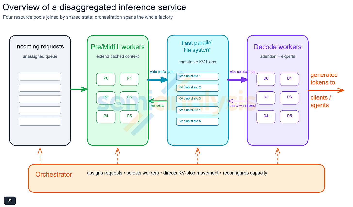
](https://substackcdn.com/image/fetch/$s_!nG_t!,f_auto,q_auto:good,fl_progressive:steep/https%3A%2F%2Fsubstack-post-media.s3.amazonaws.com%2Fpublic%2Fimages%2F0e02df36-fc57-4ee4-9015-52aa09fd7c07_2500x1470.png)Figure 1. Overview of model stages in an inference service.

1. Orchestration delivers requests via queues into pools of workers

An inference service is a cluster where prior requests and immutable state are stored when idle and then queued for delivery to specialized workers when a new request pulls in context or a prior request reawakens for continuation. The incoming queue is not yet a batch. Each request carries prompt tokens, references to reusable context, service objectives, and often an existing conversation or agent state. An orchestrator may place it into a prefill, midfill, or decode batch, and the request can join or leave that batch independently as it completes, making that capacity available for new work. Continuous batching works best when the scheduler knows which workers have slots that match the request’s context length and service objective.

Prefill workers create context from a substantial block of new tokens. Their output is new KV state for every model layer, stored independently of the worker that created it. The KV state moves along model layers, the output of layer K from one turn becomes input to layer K in the next turn. In pipelined servers this creates a natural “torrenting” of output and input from separate NICs.

Midfill workers extend previously processed context. The cached prefix may contain system and user prompts, memories, earlier conversation turns, agent steps, or retrieved documents. Large roots may be already cached, while the incremental input can be much smaller than a comparable uncached request: a half-million context may receive only a few hundred or a few thousand new tokens.

Decode workers consume the processed, accumulated context and generate one or a few tokens (multi-token prediction is becoming quite common) per pass. Every generated token adds a small amount of new state. The same context can later return to a midfill worker when a user, tool, or agent contributes another block of input. Agentic work using tools creates a repeated sequence of context extension and generation, not merely one prefill followed by one decode.

A worker may occupy a node, a tray, or a rack. The service becomes large by operating many bounded workers and moving requests and state among them. Depending on precision and working-state requirements, even multi-trillion-parameter models can fit within the aggregate memory of a modern rack-scale system. The datacenter network remains essential because the factory must connect many such workers to shared storage and continuously match worker configurations to demand. KV transfers may be gigabytes in size, but they can be striped or torrented across multiple links and destinations; their movement time can remain well below the lifetime of a long decode job.

This separation is useful for both performance and operations. Prefill and midfill are predictable once the cached-prefix size, new-token count, and worker configuration are known. Decode completion time is stochastic because arrival of the final output token cannot be predicted in advance. Shared memory and storage between the pools let each stage run at its own cadence. Later sections of this article will discuss queues, ready buffers, and worker reconfiguration. For now, the important point is that the service is a loop of stages joined by movable state.

AgentX examples

[
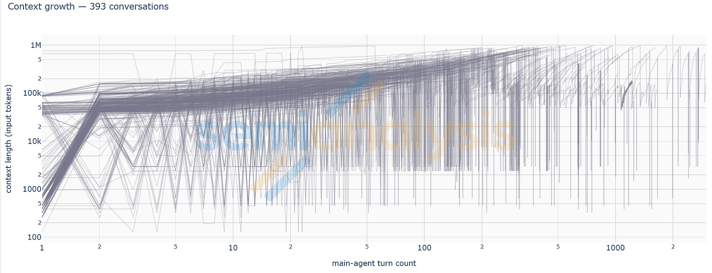
](https://substackcdn.com/image/fetch/$s_!xosE!,f_auto,q_auto:good,fl_progressive:steep/https%3A%2F%2Fsubstack-post-media.s3.amazonaws.com%2Fpublic%2Fimages%2F50dba89e-9dfd-4d9d-831c-3dcd1748a45e_2022x776.png)Figure 2. “CC Traces Weka” dataset contributed to AgentX, release 34. Source: SemiAnalysis AgentX.

This is viewed with the SemiAnalysis Conversation Explorer. It shows that context growth during conversations can be quite rapid but also goes through large fluctuations due to compaction and other model behavior which may not be explained in public discussions. Orchestration of the inference context is a competitive advantage for AI companies.

[
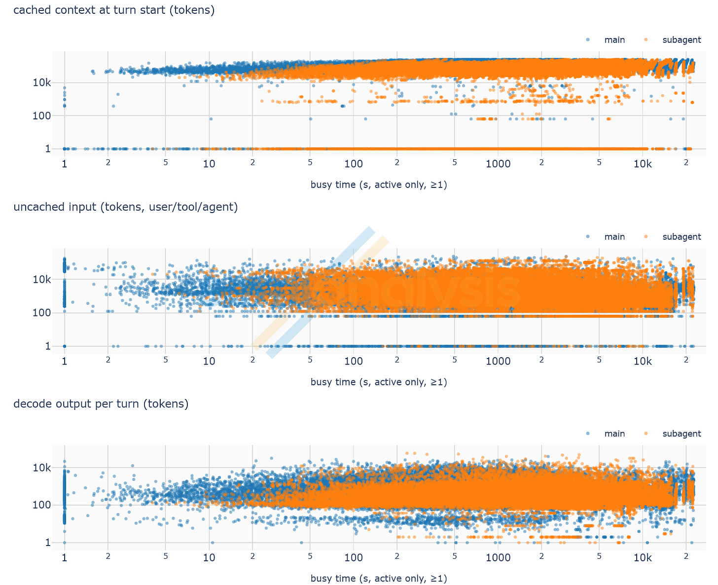
](https://substackcdn.com/image/fetch/$s_!lXqX!,f_auto,q_auto:good,fl_progressive:steep/https%3A%2F%2Fsubstack-post-media.s3.amazonaws.com%2Fpublic%2Fimages%2Fc1a155ad-ce74-4b40-a4bc-b1e4af1fa624_1510x1230.png)Figure 3. Cache, new input, and result lengths seen at each turn of the same conversations. Source: SemiAnalysis AgentX.

We can take that same dataset and pull out the cache, new input, and result length values seen at every turn. This visual shows how the Token Factory needs to serve many different workloads. In principle there could be requests similar to each dot in those traces (and more dots from other workload datasets) all running at the same time, assigned to some worker in the AI cluster.

This article aims to survey some of the major functions in inference that make it possible,

2. KV state moves as immutable blobs

Reusable context at data-center scale becomes a shared object-store of immutable blobs rather than a file attached to one machine. A system prompt, project context, previous user turns, tool output, and generated tokens can be in separate blobs. A new operation reads the blobs it needs and appends new ones; existing blobs normally remain unchanged. This forward-only structure follows the causal transformer itself. Changes can be handled by backtracking and creating a new branch rather than rewriting the common path.

The durable source of these blobs is a fast, parallel, scale-out memory and storage pool. It needs enough aggregate bandwidth and network reach that prefill, midfill, and decode workers can be selected for suitability and availability rather than because one machine owns the only copy of the context. Newly idle blobs can first move into shared network-attached DRAM, including node-CPU memory and dedicated memory appliances. As that tier fills, a classifier can discard blobs that are not likely for reuse, or promote longer-lived state to SSD. The underlying text and references are often orders of magnitude smaller than the expanded KV representation, so it is possible rebuild a KV blob from that smaller text if the triage decided to reuse space and discarded the expanded embedded state. AI calculations can vary subtly, so while the rebuilt state can be expected to be a valid context, services may take different approaches to how casually they discard and rebuild, and how much they try to keep important immutable state.

For a deeper dive on how the blobs are managed, Unified Radix Cache: One Tree for Hybrid Model Prefix Caching - LMSYS Org is recommended reading. It is not the last word, but it is clearly written and will point you to other sources if you want to look for more.

There are also frequent compactions of state with long-running agents that build up to the maximum context, so in general after a compaction there will be many prior blobs which have been abandoned in favor of a new context. The space from the pre-compaction contexts is probably recycled for new work.

[
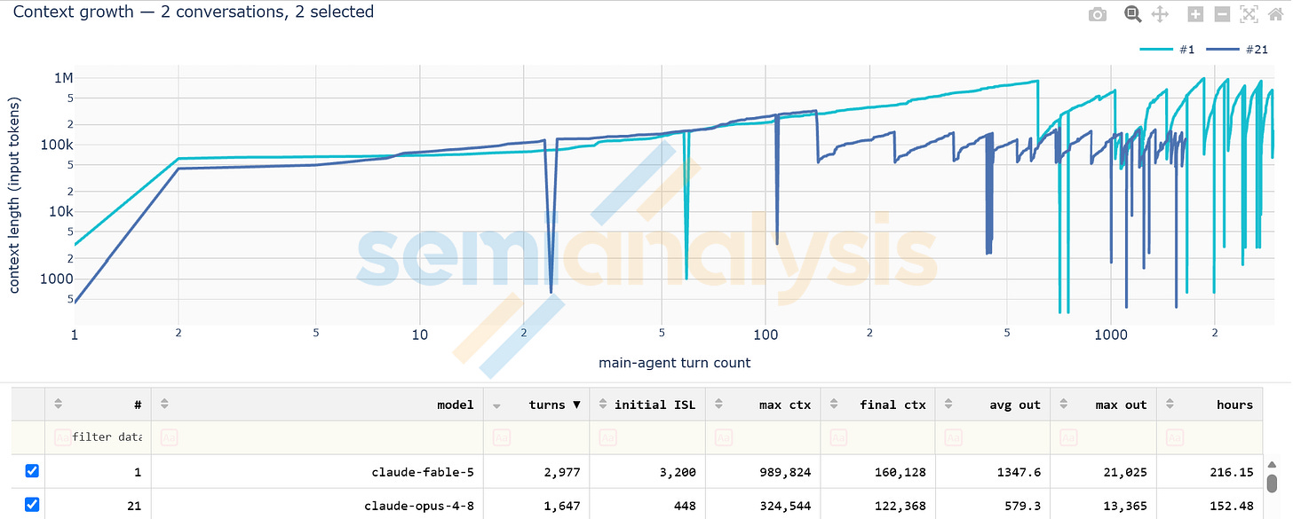
](https://substackcdn.com/image/fetch/$s_!aFGC!,f_auto,q_auto:good,fl_progressive:steep/https%3A%2F%2Fsubstack-post-media.s3.amazonaws.com%2Fpublic%2Fimages%2Fa1426880-84ea-42b8-be37-ea5e967ad662_2032x816.png)Figure 4. AgentX release 34, selected conversations. Source: SemiAnalysis AgentX.

You can see compactions occur in the right half of these conversations as contexts get close to the practical context limit for each model (250k tokens for Opus 4.8, 1MT for Fable). There are also “stalactites” in both lines which seem transient and reflect some proprietary behavior in Anthropic models.

Accelerator HBM is the “hot” working tier. It is too expensive and supply-constrained to be a good default for passive context storage. The active prefix and suffix should enter HBM shortly before use and leave promptly after the worker has finished with them. CPU DRAM is a useful staging and assembly tier, especially for outgoing state: a completed worker can move newly generated blobs into CPU memory while the storage system chooses placement and redundancy, after which the NIC sends them into the shared pool.

For incoming data, RDMA-capable systems may allow the network to place data directly into accelerator memory, avoiding a full copy through CPU DRAM. CPU memory still remains useful for metadata, coordination, partial assembly, fallback paths, replicas, and outgoing staging. When a worker uses multiple GPUs the incoming context can be striped directly to their destination memories in parallel.

Rack-level hot-blob caches can also be useful, whether implemented as memory/storage appliances or making use CPU memory which is assigned to the distributed storage pool. Very common objects such as system prompts are natural candidates. These caches should remain shared scale-out resources rather than private state that binds a request to one decode machine. HBM is several times more expensive and more supply-constrained than DDR. HBM’s best use is for data ina an active batch currently earning revenue.

[
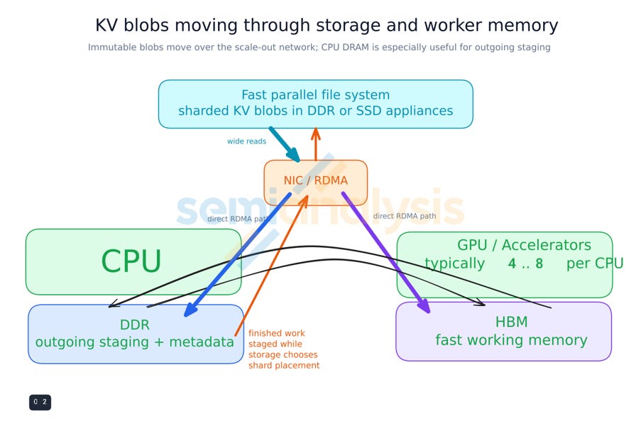
](https://substackcdn.com/image/fetch/$s_!JBSP!,f_auto,q_auto:good,fl_progressive:steep/https%3A%2F%2Fsubstack-post-media.s3.amazonaws.com%2Fpublic%2Fimages%2F6e1c09c0-f0e2-403a-83fa-b089cb442e4e_903x597.png)Figure 5. KV blobs moving through storage and worker memory.

Data input is generally larger than output. Midfill commonly reads a large prefix and appends a meaningful but smaller suffix. Decode reads the accumulated context and appends only the state for one or a few generated tokens. The reads are repeated, the writes usually occur just once. The system design should show these differences directly with the width of each data path.

3. Prefill, midfill, and decode create distinct operating regimes

The global service contains several computational regimes. Their differences are more useful than the generic labels compute-bound and memory-bound, because each has a different opportunity for reuse and a different natural mapping onto hardware.

3.1 Prefill

Classic prefill begins with little or no reusable KV state and processes a substantial block of new tokens. Those tokens share weight loads, use matrix operations efficiently, and create enough routed activations to form useful shared-expert batches. Attention and dense transforms can reach high arithmetic intensity, so prefill is often constrained primarily by compute. Long initial input contexts can raise memory traffic but these rarely get to 100,000 tokens in length, while midfill is commonly beyond that.

3.2 Midfill

Midfill appends new tokens to a much longer cached prefix. The new block can still provide hundreds or thousands of activations for shared weight and expert reuse, raising arithmetic intensity to thousands of ops per byte of data. Attention must also read a large existing KV state, which can be tens of GB. It therefore sits in a mixed regime: more arithmetic reuse than decode, but much more cached-state traffic than an initial prefill of the same new-token count.

3.3 Decode attention

Decode advances on input of one or a few tokens per query. Each query brings its own KV state which is similar in length to what midfill processes. While prefill differs from midfill on length of cache, decode differs from midfill in input sequence length. These one to few input tokens keep arithmetic intensity low, this work is clearly dominated by the memory movement around the KV cache.

For long contexts, the attention read can exceed the size of tensor operations associated with model weights. Attention is therefore one of the largest operations in modern decode even though most model parameters reside in experts. Delta, top-k, or linear-attention algorithm layers can reduce the burden, but periodic use of a layer with full attention remains a major memory load. Each query brings its own context, so batching queries does not change the arithmetic intensity of attention.

3.4 Decode experts

Experts are not specific to the decode phase. Everywhere the model runs the experts run, and they require no context other than one token’s embedding. The history of the query has already been compressed into the activation presented to the expert. This allows various designs that share the experts across all available GPUs, reducing memory size per GPU and increasing the memory bandwidth / memory size, or memory intensity ratio. You can look at the interval needed for a GPU to read all its experts as the best case interactivity (token rate seen by each user) and so if the memory bandwidth remains constant but the GPU is responsible for fewer experts, interactivity can be higher. The gotcha is that networking needs also rise, and the all-to-all pattern needed for routing to experts is a difficult one.

At the end of attention (in prefill, midfill, or decode) a router calculation (a small tensor operating on the unrefined token) selects a few experts for each new token. Tokens that select the same expert can share a tensor-weight load even when they come from different requests, so long as they can be gathered together in time to take advantage of the same weight loading. In practice their may be 15,000 experts across all the layers, so taking advantage of such coincidences requires deliberate synchronization like awaiting until all queries in a batch have completed attention until switching over to sending them for expert work, and that in turn may be improved by having multiple instances in different nearby machines also synchronized to that schedule. If you have ever wondered why Nvidia makes such an effort to connect 72 GPUs so closely, this is a big part of why. In a large token factory it is feasible to have those 72 machines all running in sync, allowing the experts in one layer to be divided up to 72 ways. If a layer of the model has 256 experts then each GPU is handling only 3 or 4 in each layer, permitting very fast complete cycling through all the experts. And a lot of all-to-all traffic.

Something interesting happens if your experts can all be kept in SRAM. You need a huge number of accelerators and a monster network to collect them all to all back to the GPUs, but now there is little reason to wait for a batch to form. Each expert can run whenever it has input. The energy per byte loaded is as much as 100x better than loading from HBM, so a single token running can be as efficient as perhaps a queue of 100 was before. In return for this DAF (disaggregated attention-FFN, where the experts are the FFN) you can free up the instances from needing to be synchronized. This advantage does not help as much with prefill or midfill since they trivially have a batch of tokens they can sort into shared queues on one layer, but it still may offload all the expert weights from those GPUs allowing them to optimize their local memory for other uses like longer contexts. The networking is still a gotcha, where an SRAM based accelerator could turn around an expert calculation in less than a microsecond but now you may be flooding a switch connected to hundreds of nodes with the all to all traffic for millions of tokens. The network may absorb more money and power than the experts they connect.

[
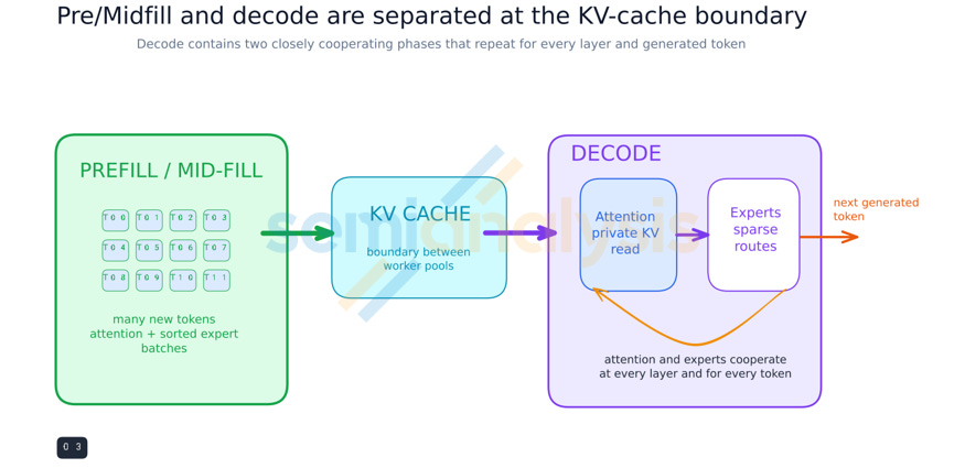
](https://substackcdn.com/image/fetch/$s_!0swW!,f_auto,q_auto:good,fl_progressive:steep/https%3A%2F%2Fsubstack-post-media.s3.amazonaws.com%2Fpublic%2Fimages%2F132a56e8-d9e0-42cd-bcda-5051cab4b9b3_875x425.png)Figure 6. Prefill and midfill are separated from the closely coupled decode loop at the KV-cache boundary.

Inference workers can improve sharing by coordinating many attention instances on the same model layer. Their routed activations then draw from one layer’s expert bank, reducing the number of different experts each destination must load. In a pipelined server this also means the networking connections used for expert parallel can be local to that stage of the machine, there will never be a routing that needs experts from another layer. Even so, each decode request contributes only one new token with typically 8 to 16 routed experts per pass, and a layer may contain hundreds of experts. At small batches, sharing remains limited and memory bandwidth continues to dominate both the KV scan and the active expert loads, with very little computation per byte of weight loaded. Expert memory needs to be very low energy per bit, no matter what kind of memory is in use.

These regimes explain why prefill, midfill, and decode may prefer different worker configurations; why decode attention and decode experts can prefer different placements within a node; and why batching helps each stage by a different amount. As prefill in modern agent work rapidly expands to the 500k token range there is a lot of memory movement, especially in token decode - the stage where the model is generating useful intermediate and final results. Fast and large 3D RAM will be decisive in efficiency. Fast memory is also useful for midfill. However, capacity needs to reach a minimum level for the large contexts we now see as normal. If memory capacity is too small then the losses in networking and excessive swarms of chips can waste power compared to future memory types which will use 3D capacity expansion without giving up on throughput.

[
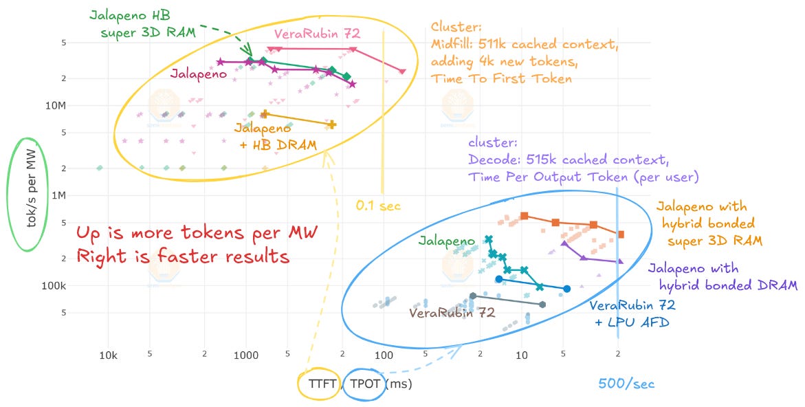
](https://substackcdn.com/image/fetch/$s_!zjGq!,f_auto,q_auto:good,fl_progressive:steep/https%3A%2F%2Fsubstack-post-media.s3.amazonaws.com%2Fpublic%2Fimages%2Fa138a4da-0245-453d-8d93-dbeca158f2f6_1171x592.png)Figure 7. Projected effect of faster memory (hybrid-bonded DRAM, super-fast 3D RAM)) on midfill and decode with 500k token context cache length. Source: SemiAnalysis model simulator with projected accelerator and GPU performance.

While Vera Rubin 72 can crush at the mid-fill layer, which is arithmetic intense, it is not so effective at the switch to memory intensive decode where the Rubin cannot fully exercise its computational prowess. With the large context there is a premium on keeping the decode work in the same node and the midfill, avoiding sending the context across the network to a different node. This could favor an all-around chip which both has super memory thruput and really efficient computation.

4. Flow through an MoE prefill layer

Classic prefill begins with attention. A block of new query tokens attends to reusable prefixes like the system prompt and to earlier positions in the new block. The attention operation produces one activation for every new token, and shared transformations prepare those activations for the routed-expert stage.

The router assigns several experts to every token. If the model selects eight routed experts, each incoming token produces roughly eight routes across a bank that may contain 256 experts or more. In token order, those records are sparse and interleaved: neighboring tokens can have completely different destinations. Across the full input block, however, every expert can accumulate a short list of assigned tokens.

The worker sorts or queues the route records by expert identifier. All activations assigned to expert 037 become one message stream; those assigned to 142 become another. A single expert-weight load can then serve all activations in that bucket. Several requests can contribute to the same buckets, and separate attention instances running the same layer can merge their routed work at the expert destination. Converting token order into expert order is one of the central efficiencies of MoE prefill. Scale-up networks like NVLink can be organized as memory mapped connections so sending requests to specific experts could be mapped to pushing the message into a specific memory mapped location which is configured as a hardware queue. There is very little start and stop time. The experts can listen with the equivalent of an RDMA CIQ that again leverages hardware acceleration to deliver the message stream without need for complex protocol start and stop. Simple headers inline on the message identify the sender and receiver. A similar connection can be set up for the return flow from expert back to the decode worker.

The expert outputs are returned to token order, weighted, combined, and passed to the next layer. At the same time, attention creates new K and V state for the appended tokens. Across the model, those values form an immutable KV suffix which are used to decode the next token, and which are eventually stored as the next blob in the context for use by the next turn in the conversation.

Prefill therefore combines two forms of weight reuse. Attention and dense transforms reuse weights across many tokens, while routed experts reuse each selected expert across the tokens collected in its bucket. The gains eventually flatten as growth in activation traffic, KV traffic, and output handling take more time compared to the tensor calculations. Batching can delay time to first token, but a single request containing several thousand new tokens already provides substantial arithmetic intensity; prefill does not always need a large number of requests in each batch to run efficiently. Modern single-socket GPUs may be able to do the prefill even on a large model for a small batch in around a second.

[
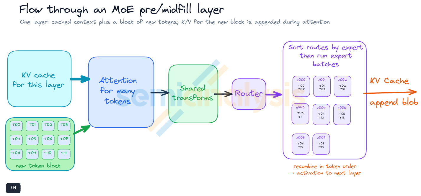
](https://substackcdn.com/image/fetch/$s_!OrHW!,f_auto,q_auto:good,fl_progressive:steep/https%3A%2F%2Fsubstack-post-media.s3.amazonaws.com%2Fpublic%2Fimages%2F8405f00c-c10b-41b8-b2f8-c3e4dfd7b136_1426x665.png)Figure 8. Flow through an MoE prefill layer.

5. Flow through an MoE decode layer

Decode begins with a much smaller amount of new work per forward pass. The current token, or a handful of speculated tokens in MTP (multi-token prediction) is the query. Attention reads the prior KV state together with the new token’s KV entry. The new entry appends to the result and is appended to the KV state for the next pass.

For agentic contexts, the prior KV state is often a heavier read burden than the attention and expert weights used by that one token. The new query and its local projection weights are comparatively compact. Attention may be partitioned across KV heads, context ranges, memory channels, or accelerator units, after which partial results are reduced to one token activation. That activation is small enough to move cheaply even though it will trigger much larger local tensor operations in the next phase.

The activation passes through shared transformations and routing. The router selects a few experts from the available bank, and only those expert tensors become active for the current token. Their outputs are weighted, combined, projected, and passed onward.

At each layer, attention creates and retains that layer’s K/V entry for the new token. The activation then advances to attention in the next layer, where the same sequence repeats. By the time the final layer produces the next token, every layer has appended its small K/V update. Those updates can be assembled into a new immutable KV suffix while the token is streamed to the client or agent.

The flow therefore contains both a broad operation and a sparse operation. Attention reads widely across private query state. Experts activate a small subset of total model capacity. The hardware mapping should support both without forcing the entire layer to use one parallelism strategy.

[
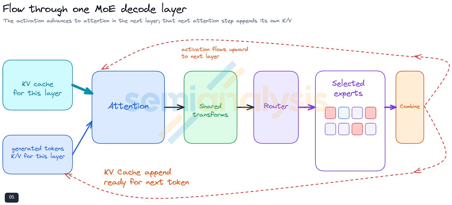
](https://substackcdn.com/image/fetch/$s_!lj9A!,f_auto,q_auto:good,fl_progressive:steep/https%3A%2F%2Fsubstack-post-media.s3.amazonaws.com%2Fpublic%2Fimages%2F2c316fba-4573-4690-b119-d8416000b55c_1621x737.png)Figure 9. Flow through one MoE decode layer.

6. Midfill is a distinct operating regime

Midfill combines a long, cached prefix with a block of new tokens to prepare another turn in a conversation or agentic work. Traces show the cached input to be many times larger than the incremental query, although the incremental query typically varies from 50 to 5,000 new input tokens. The presence of cached system prompts, conversation roots, memories, prior agent steps, and retrieved documents can quickly raise conversational and agentic contexts to a million limit. AgentX datasets show frontier experts are repeatedly compressing contexts to stay under a million-token limit.

This makes midfill neither a small prefill nor a large decode. Like decode, it must read a substantial private KV cache. Like prefill, it processes enough new tokens to reuse weights and to sort routed activations into useful expert batches. Its arithmetic intensity can be hundreds of times greater than one-token decode, yet its cached-state traffic can be tens of times larger than that of a similarly sized initial prefill.

Modern accelerators can generally exploit the arithmetic reuse available in a block of hundreds of tokens, so the difficult balance is often between the large KV read and the burst of routed-expert traffic. That burst does not match the smooth rhythm of a decode pipeline: a midfill can occupy a stage much longer than the decode batches in neighboring stages, leaving those stages underused.

The ideal parallelism can also differ. The worked example later in this essay finds midfill configurations that use different pipeline, tensor, and expert-parallel settings from decode. Reconfiguring a GPU in the middle of a live decode pipeline can be expensive or impractical. A service may therefore benefit from a dedicated pool of midfill-optimized nodes. The hardware can be identical to the decode pool while the loaded model stages, parallelism, and batch policies differ.

[
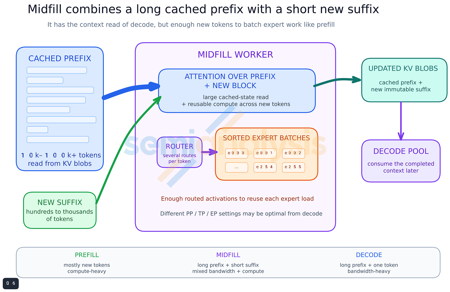
](https://substackcdn.com/image/fetch/$s_!9Kjl!,f_auto,q_auto:good,fl_progressive:steep/https%3A%2F%2Fsubstack-post-media.s3.amazonaws.com%2Fpublic%2Fimages%2F87a47cb2-ded5-4daa-b7e0-6eb17ce03340_3100x2012.png)Figure 10. Midfill combines the cached-state read of decode with enough new tokens to batch model and expert work.

7. The model is a tall stack of repeating layer groups

A model’s parameter count quantifies the total learned state, but serving depends on how that state is organized and used. The model is a stack of layers, and increasingly it is useful to group those layers into repeating architectural units.

In some MoE models, a layer group is the same as one layer. In others, a group contains one full-attention layer together with several linear, delta, top-k, or otherwise optimized-attention layers. Typically 1 to 3 of the initial layers may be dense or otherwise designed to get a clean start. The rest of the model will normally repeat one recurring group pattern.

A wide, shallow crêpe is a useful representation of a layer group. The broad surface provides room for attention, shared transforms, routing, expert capacity, and residual flow. Its shallow thickness marks the group as one slice in a much taller repeated model. It also echoes the physical form of an accelerator: a very thin active layer spread across a broad package. The crêpe is a useful intuition for mapping a wide algorithmic flow onto a wide hardware surface.

The repeated structure simplifies function planning. A mapping created for one group can be reused for the next. Corresponding memory regions can hold the next group’s weights. The same compute and communication plan can execute repeatedly. Uniformity matters not only for runtime efficiency but also for compiler, kernel, and operations tooling.

[
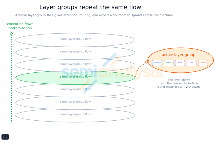
](https://substackcdn.com/image/fetch/$s_!NvYr!,f_auto,q_auto:good,fl_progressive:steep/https%3A%2F%2Fsubstack-post-media.s3.amazonaws.com%2Fpublic%2Fimages%2F0f20bc9d-d860-4e6d-8387-5e2ba79e9bf2_732x478.png)Figure 11. Layer groups repeat the same flow.

During decode, one layer is active at a time for a given token. Within that layer, several operations occur sequentially. Neighboring layers may be prefetched, and different pipeline stages may process different queries simultaneously, but the logical path of one token still climbs through the stack in order.

[
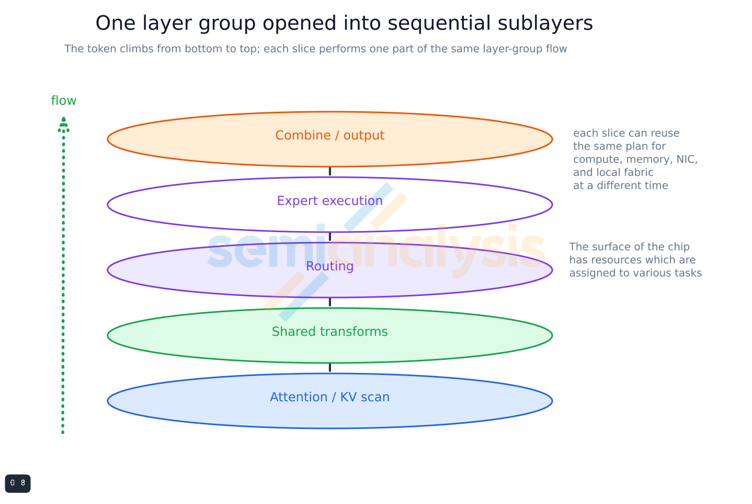
](https://substackcdn.com/image/fetch/$s_!RRxu!,f_auto,q_auto:good,fl_progressive:steep/https%3A%2F%2Fsubstack-post-media.s3.amazonaws.com%2Fpublic%2Fimages%2F1cf97cc6-a4b5-403e-b115-97845e79b636_752x504.png)Figure 12. One layer group opened into sequential sublayers.

8. Parallelism should partition the narrow dataflows of the model

Parallelism is not one decision. Pipeline, tensor, and expert parallelism divide different dimensions of the model and should be judged by different communication patterns.

Pipeline parallelism follows the layer stack

Layers immediately suggest pipelining. The activation passed between layers is compact—often one embedded token, a small multi-token-prediction block, or brief summaries of prior hybrid group results —while the weights and KV state used inside a layer are much larger. A pipeline stage can therefore own one or more complete layer groups and pass a relatively small activation to the next stage without overpowered networking.

Pipelining divides model weights cleanly and keeps hot within-layer communication local. Its main drawback is multi-batch occupancy: a fully active pipeline has a different query or batch in every stage. Each stage therefore holds its share of the KV state for all live streams, and the memory benefit eventually stops improving as contexts grow.

Tensor parallelism belongs where one operation is intrinsically broad

Attention may need to divide weights and KV state across several accelerators. KV heads, context ranges, or another linear dimension can be partitioned so that each accelerator processes its share before a compact reduction of the token result. Tensor parallelism can also serve unusually large dense transforms.

TP should not spread automatically into every tensor of the layer. A collective that is sensible for a broad attention operation may cost more than the arithmetic of a small expert tensor.

Expert parallelism follows independent expert tensors

Most MoE parameter memory may reside in experts. Experts retain no query history of their own; context arrives in the activation. The expert bank can therefore be distributed widely across a peer set and shared by several worker instances.

Wide expert parallelism is useful because the experts are independent and numerous. The router sends compact activations to selected destinations, and those destinations return transformed activations. Expert-parallel width can remain large even if pipeline stages become smaller, allowing switch radix and local memory placement to be chosen independently.

The general rule is straightforward: use pipeline parallelism for the vertical layer sequence, tensor parallelism for large indivisible operations, and expert parallelism for the context-free routed-expert bank. A stage fits comfortably inside a scale-up domain when its available fast memory safely exceeds its local weights, live batch state, and working buffers:

M_{free,node}>\frac{W}{P}+M_{batch}+M_{working}

Modern GPU nodes often exceed that threshold by multiples. When they do, the demanding bandwidth, power, and latency requirements can remain inside one node while thinner pipeline activations and KV movement use scale-out links. The rest of the fast memory is probably not earning any revenue. Data sitting idle in memory is an expense, data moving to be processed is revenue.

[
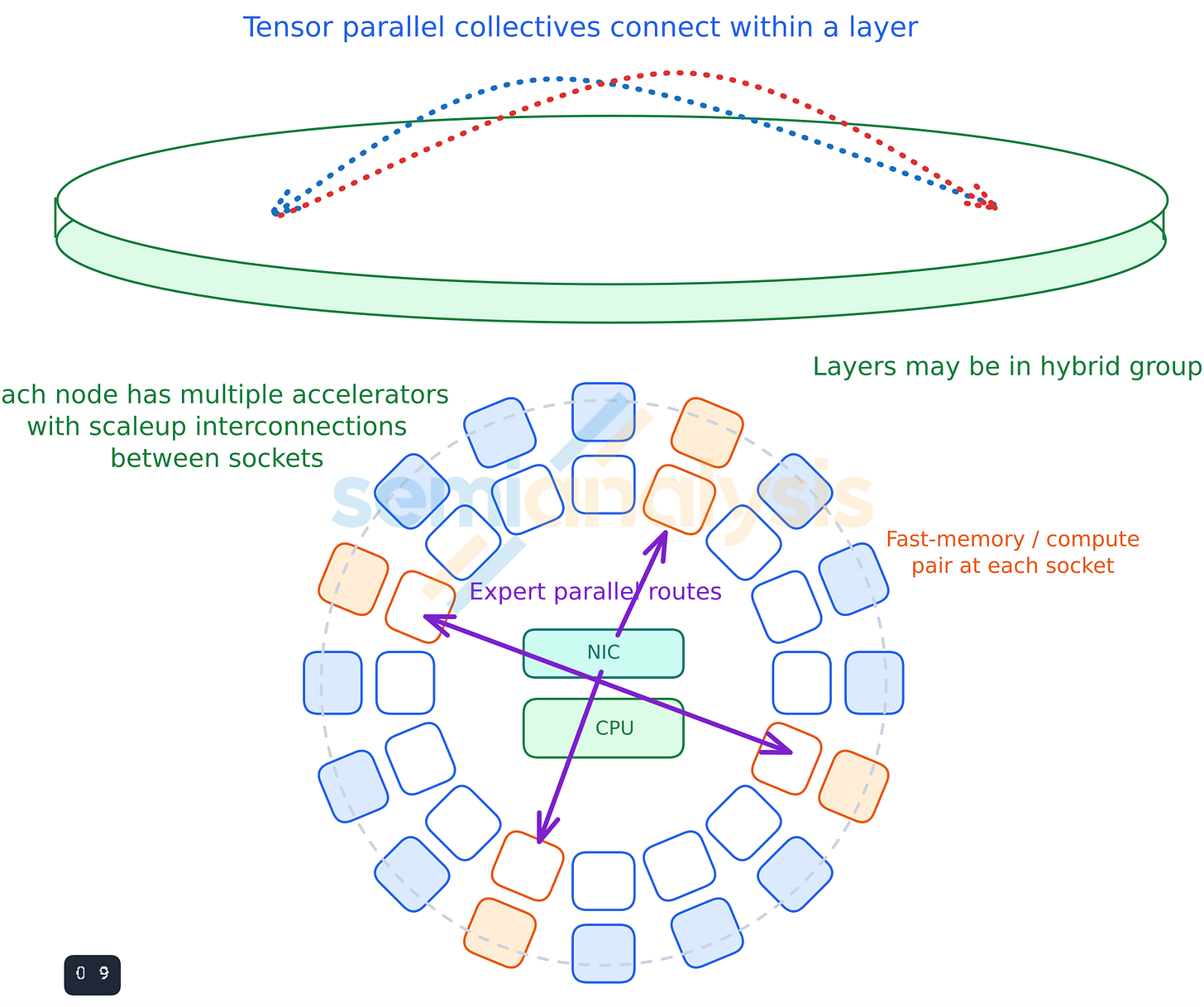
](https://substackcdn.com/image/fetch/$s_!bgFY!,f_auto,q_auto:good,fl_progressive:steep/https%3A%2F%2Fsubstack-post-media.s3.amazonaws.com%2Fpublic%2Fimages%2F092167fa-cb58-4f8e-a168-1c60bf339415_2079x1739.png)Figure 13. Pipeline, tensor, and expert parallelism follow different dimensions of a layer group.

9. A logical accelerator node

A logical node is easier to understand as a peer set arranged in a ring than as a literal circuit-board layout. The ring contains perhaps sixteen accelerators. Each accelerator pairs a compute region with local fast memory. The units connect through a strong scale-up fabric. A CPU coordinates workload and memory management, while a NIC connects the node to rack and datacenter resources.

The ring is just a visualization which shows the accelerators as peers, with equal standing. I am not implying the node-internal network should be a ring. It could be hub and spoke, rail, all-to-all, torus, hypercube .. whatever floats your boat, so long as it can handle the highest dataflows the rack contains with low latency and low energy per bit. I’ll just draw it as a ring for simplicity.

This representation avoids committing too early to package placement, board routing, or switch implementation. The actual machine may use a central switch, several switches, direct links, or a hierarchical fabric. The logical requirement is a bounded peer set with predictable fast local communication.

The accelerator design may vary. One version may use SRAM-heavy processing-in-memory units. Another may use hybrid-bonded DRAM, or IGZO memory cells placed on top during BEOL processing. Another may use a hybrid-bonded high-bandwidth true 3D memory. Memory capacity and bandwidth can change while this logical model remains useful.

The node is the natural place to keep work that repeats at high frequency. Attention partitions exchange compact partial results. Routed expert activations travel to local destinations. Expert outputs return for recombination. Shared state and scheduling metadata remain near the CPU. The NIC carries pipeline activations, KV blobs, and work assignments beyond the node.

A node may be smaller than a rack like we see in an SGX node with 8 GPUs, or a scale-up system may span the whole rack like we see with NVL72. The logical symbol remains valid in either case. If scale-up already covers the rack, the separate rack-backbone level disappears and the next boundary is directly to scale-out networking.

[
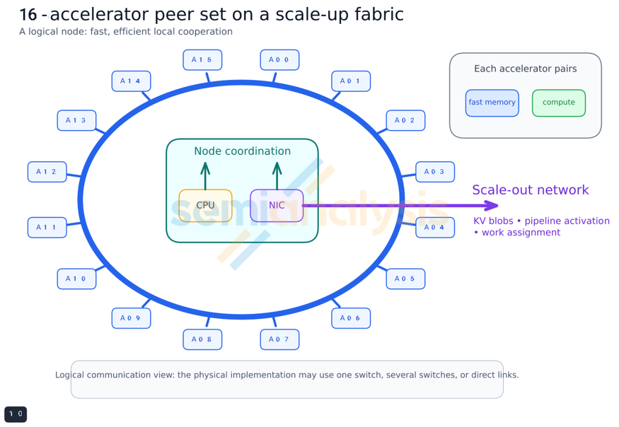
](https://substackcdn.com/image/fetch/$s_!5yYB!,f_auto,q_auto:good,fl_progressive:steep/https%3A%2F%2Fsubstack-post-media.s3.amazonaws.com%2Fpublic%2Fimages%2F3ff6ec22-e5fb-405a-8165-4a6b44c92198_875x604.png)Figure 14. A 16-accelerator peer set on a scale-up fabric.

10. Nodes stack to make racks

The ring becomes more expressive when tilted as broad, shallow hardware crêpe. Several units can be stacked vertically in a rack, like model layer groups stacked in model depth.

This repeated form makes the model-to-hardware relationship easier to see. A layer-group crêpe can be placed onto one hardware crêpe. Several layer groups can occupy one node if memory permits. One layer group can span several tightly connected nodes if attention or expert capacity requires it. The mapping can expand or contract without changing the basic visual vocabulary.

A rack may be organized in several ways:

one rack-wide scale-up domain;

several node-scale islands connected by a rack backbone;

pipeline stages distributed among those islands;

wide expert placement within each stage;

or a mixture of stage-local scale-up and shared scale-out links.

The rack backbone is therefore an optional middle level. Some systems extend the scaleup fabric across the rack needing no separate node connector. Others use strong local node fabrics and a distinct top-of-rack or shared-rail network. Above the rack, scale-out networking connects storage, prefill pools, decode pools, and other racks.

The repeated rack units also help separate two kinds of scale. The model can fit within one bounded rack worker, while the factory scales by adding many workers. The first problem is function placement. The second is worker orchestration.

[
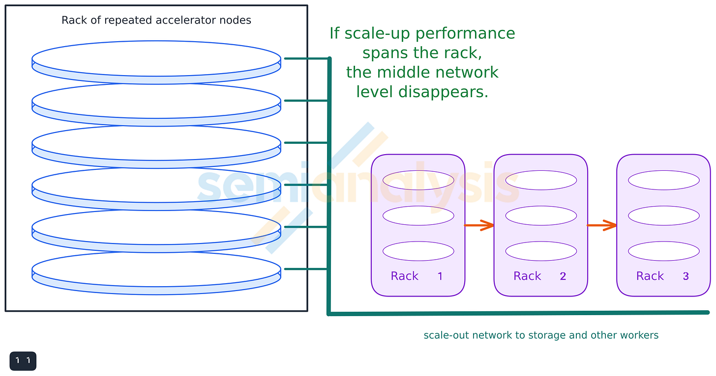
](https://substackcdn.com/image/fetch/$s_!9JtJ!,f_auto,q_auto:good,fl_progressive:steep/https%3A%2F%2Fsubstack-post-media.s3.amazonaws.com%2Fpublic%2Fimages%2F69500e04-c899-42bb-afd9-854d41716196_2614x1376.png)Figure 15. Accelerator nodes stacked into a rack.

11. One layer group reuses the node over time

A layer group does not require every operation in the algorithm at peak intensity simultaneously. Its operations form a repeating sequence that reuses the same hardware for different work over the decode cycle.

Attention may spread across much of the ring, using many memory channels and several compute units. The query and output transformations use model weights in more compact operations. Shared feed-forward work may use a dense region. Selected experts then activate local memory-and-compute regions around the ring. Recombination returns a compact result.

The same physical accelerators can participate differently at each step. Execution units that calculate attention may later execute one or more experts. Memory channels used to stream KV state can later feed expert weights. Buffers and local links are reused as the token advances.

This time-sharing is central to an efficient design. Static diagrams can make the machine appear underused because not every block is active at once. In reality the hardware is serving a sequence of different operations, and the goal is to keep the sequence moving with little setup or synchronization overhead.

The broad layer-group crêpe and the accelerator peer set are complementary. The crêpe shows the algorithmic flow; the ring shows the reusable physical resources beneath it. Mapping is the act of aligning each stage of the flow with a suitable subset of the ring.

[
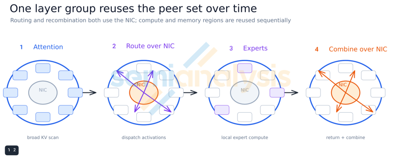
](https://substackcdn.com/image/fetch/$s_!NjGC!,f_auto,q_auto:good,fl_progressive:steep/https%3A%2F%2Fsubstack-post-media.s3.amazonaws.com%2Fpublic%2Fimages%2F20777839-1d23-4fd0-8474-75f9dd6c7835_821x325.png)Figure 16. One layer group reuses the peer set over time.

12. Put throughput boundaries where the flow is smallest

Once the model and machine are drawn as connected flows, the placement rule becomes clear: frequent, latency-sensitive communication should remain inside the strongest local fabric, while weaker links should carry compact or amortized transfers.

[
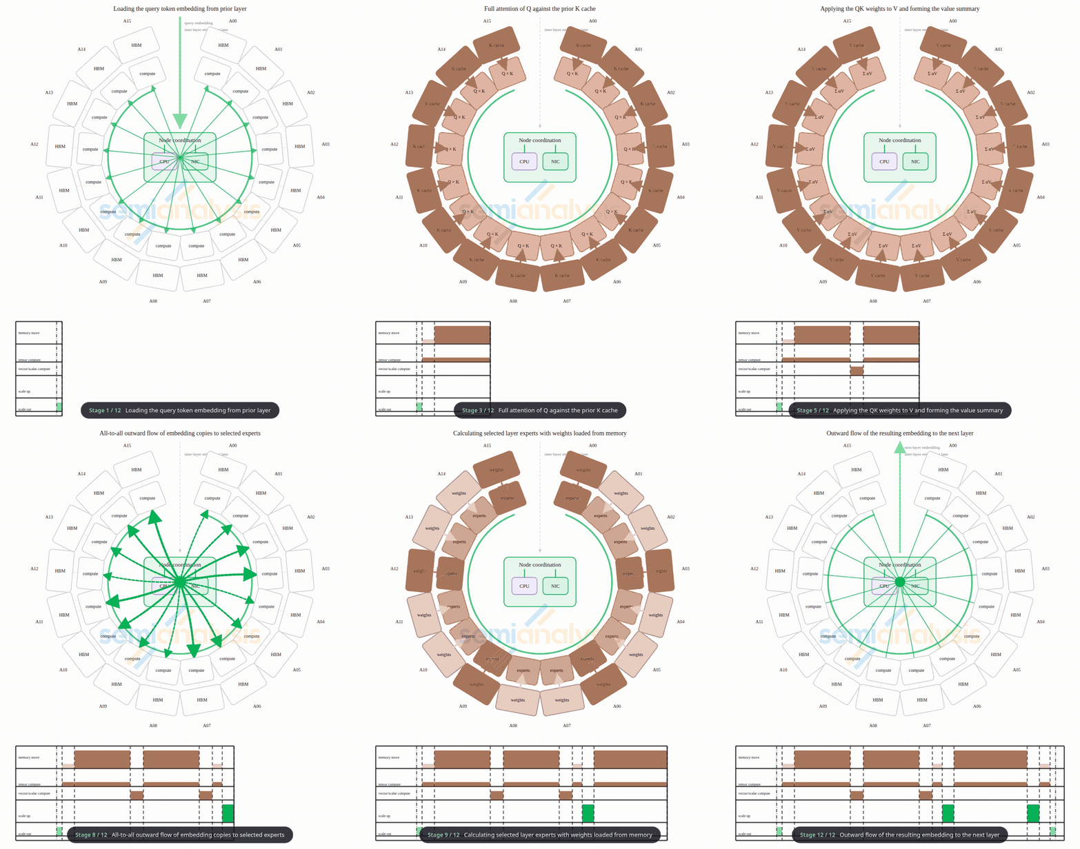
](https://substackcdn.com/image/fetch/$s_!3hdE!,f_auto,q_auto:good,fl_progressive:steep/https%3A%2F%2Fsubstack-post-media.s3.amazonaws.com%2Fpublic%2Fimages%2Ffaccb4c8-8dad-4d10-b414-ac79c068e9bd_800x944.gif)Figure 17. The general flow of operation of an MoE pipeline stage (animated).

Attention partitions may exchange partial results every layer. Expert routing sends activations to selected experts and returns their outputs. This traffic is not always the largest by byte count, but it is frequent, bursty, and sensitive to synchronization. It belongs inside the chosen scale-up domain whenever practical.

The activation passed between layers or layer groups is much smaller. A pipeline boundary can therefore cross a weaker link without moving the layer’s full internal working set. KV blobs are larger, but they move at worker boundaries and are amortized across many generated tokens. Their path can use striped or torrented scale-out networking and shared storage rather than consuming the innermost tensor fabric.

The router-to-expert boundary is typically a medium-throughput all-to-all carrying compact activations. Its difficulty often comes from endpoint count, synchronization, and routing efficiency rather than raw byte volume. Keeping it within the scale-up domain of a node or rack limits both latency and operational complexity.

This hierarchy is easier and cheaper to build than a machine in which every link is equally strong. Scale-up paths surround the operations that exchange embeddings and partial results within every layer. Scale-out links carry pipeline activations, KV movement, scheduling traffic, and traffic between bounded workers.

The tiers also have different latency requirements. A pipeline transfer between layer groups may barely notice a few microseconds if throughput is sufficient. By contrast, when an expert load and multiply take only a few microseconds, an additional 100 ns at each routing hop is material. The closest links should therefore be integrated tightly with the accelerator fabric, while less frequent transfers can tolerate the scale-out network.

13. Pipeline by layer group where practical

The layer group is the natural first candidate for pipeline placement. In a classic MoE model the group repeats one kind of layer. In newer structures it may contain one full-attention layer followed by several optimized- or localized-attention layers.

Keeping a group together can preserve internal dependencies and allow one placement and compilation plan to repeat across stages. Uniform plans reduce tooling cost and simplify deployment. Kernels, memory layouts, communication schedules, monitoring, and failure recovery all become easier when each stage runs the same recurring structure.

It is still possible to cut a pipeline in the middle of a group, although the resulting placement is more complex. If the layers have no special cross-layer dependency, the compact activation boundary remains a low-volume link suitable for networking. A stage may contain several whole groups, one group, or part of a large group depending on memory and throughput requirements.

The guiding principle is not an absolute prohibition on splitting groups. It is to prefer regular boundaries and to understand when a nonuniform split is worthwhile. Tooling and operational simplicity can be as important as a small theoretical placement gain.

[
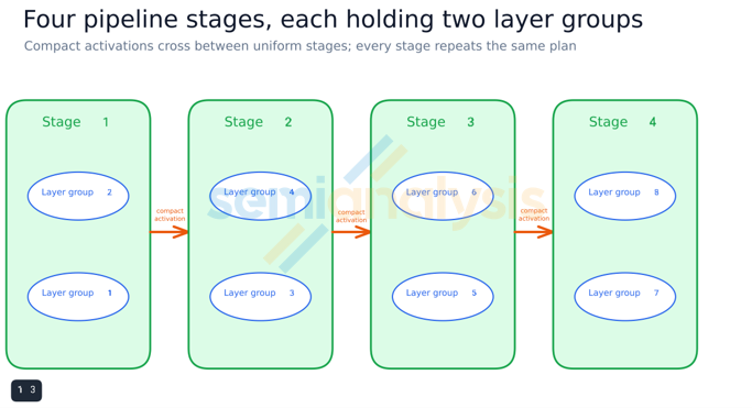
](https://substackcdn.com/image/fetch/$s_!jQh6!,f_auto,q_auto:good,fl_progressive:steep/https%3A%2F%2Fsubstack-post-media.s3.amazonaws.com%2Fpublic%2Fimages%2F1a4e2dcc-aaaf-4577-9cc4-15ea1fecab2c_683x371.png)Figure 18. Four uniform pipeline stages.

14. Pipeline depth ends at the KV-cache crossover

Pipeline parallelism divides model weights cleanly. If a model has weight footprint (W) and uses (P) stages, the idealized weight footprint per stage approaches (W/P).

KV-cache demand behaves differently. A full pipeline remains occupied by running a different query or batch in every stage. In an eight-stage pipeline, each stage owns one eighth of the layer-wise KV values for each of eight live streams. The reduction in layers per stage is offset by the number of simultaneous streams, so the stage does not receive the same (1/P) reduction in live KV demand that it receives for weights.

A useful stage-memory estimate is:

M_{stage}\approx \frac{W}{P}+M_{KV,stage}+M_{working}+M_{slack}

Once weights per stage fall to the same order as KV and working-state memory, deeper pipelining produces little additional capacity benefit while adding coordination and latency.

The crossover depends strongly on model design. Classical full-attention approaches can require hundreds of kilobytes of KV state per token across all layers. MLA-like designs are commonly in the tens of kilobytes, while recent hybrid layer groups with mostly linear, recurrent, or local attention can be lower still. A working average near 25 kB per token may be reasonable for some new hybrids; approximately 70 kB per token is a conservative reference point for a proven compressed-attention design.

As a back-of-the-envelope design target, take 70 kB per token and two million tokens of aggregate live context assigned to one stage. That is roughly 140 GB of KV state. Double buffering allows one working set to move while another continues to run, raising the KV allowance toward 280 GB. Add model weights, activations, transient buffers, routing tables, fragmentation, and operating margin, and a stage target of roughly 400–500 GB of local fast memory becomes a useful 2027 benchmark.

Other designs can reduce requirements through streaming, compression, partial residency, or additional tiers. The estimate is not a universal requirement; it is a standard that a practical frontier system should be able to accommodate without heroic assumptions.

The stage can distribute this memory over several accelerator sockets if they share a scale-up fabric. More than 95% of the weight memory in a large MoE is in routed experts, which divide naturally among sockets. KV state can be partitioned by head, context, or attention instance, with the resulting collectives matched to the same local fabric.

[
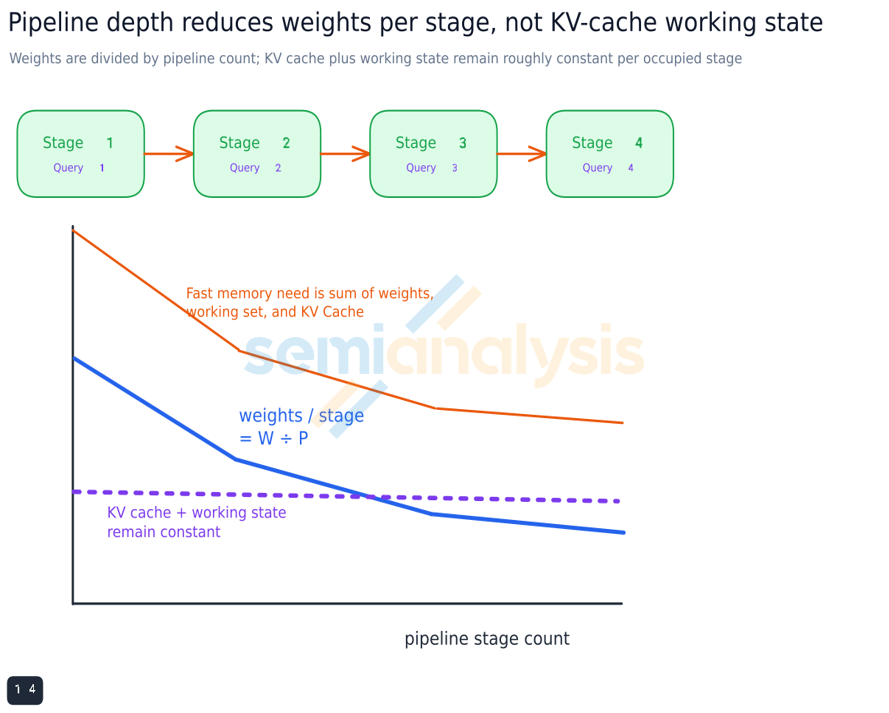
](https://substackcdn.com/image/fetch/$s_!ERxU!,f_auto,q_auto:good,fl_progressive:steep/https%3A%2F%2Fsubstack-post-media.s3.amazonaws.com%2Fpublic%2Fimages%2F4bb0253c-ef2c-4d77-83f9-e4724706da44_889x713.png)Figure 19. Fast-memory demand is stage weights, live KV state, working buffers, and margin.

15. Prefill and midfill turn sparse routes into dense expert batches

Prefill and midfill have strong batching opportunities because many input-sequence tokens complete attention before expert execution begins. The router can score all tokens, emit several destinations for each one, and then sort the route records by expert.

A practical input block can contain enough assignments that essentially every expert receives work. If 128 new tokens each select eight experts, the router emits 1,024 assignments across a 256-expert bank. Routing remains sparse for each token; sorting changes the execution order so that expert e000 processes all of its assigned tokens, then e001, and so on. Each expert is loaded once and reused for its compact token list instead of being repeatedly loaded in token order.

For an expert with (W) weights, weight traffic (B_W), activation traffic (B_A) per routed token, output traffic (B_O), and (n) assigned tokens, a rough arithmetic-intensity expression is:

AI_{expert}\approx \frac{2nW}{B_{W}+nB_{A}+B_{O}}

When weight traffic dominates, increasing (n) rapidly improves reuse. Eventually activation, output, and routing traffic become important and the gain flattens.

The sort is not free. Route records must be built, counted, permuted, sent to expert destinations, and restored to token order. Expert capacity limits can cause overflow or rerouting. Even so, prefill and midfill begin with enough tokens that the optimization is usually meaningful.

This is the key distinction from decode. The experts are identical; what changes is the number of routed activations available when the worker executes them.

[
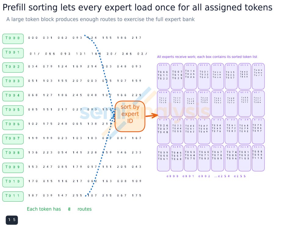
](https://substackcdn.com/image/fetch/$s_!Om5H!,f_auto,q_auto:good,fl_progressive:steep/https%3A%2F%2Fsubstack-post-media.s3.amazonaws.com%2Fpublic%2Fimages%2F55f61e24-3c24-48f9-b682-8723d3323571_950x743.png)Figure 20. Sorting lets each expert load once and process every token assigned to it.

16. Decode gains less from batching

Decode attention receives little direct cross-query reuse. Each additional query contributes another KV cache and another context scan. Shared query-projection weights can be reused, and software overhead can be amortized, but the dominant long-context read remains private to the query.

Decode experts offer potential sharing because the expert weights are context-free. The practical limitation is sharing probability. A model may contain hundreds of routed experts in every layer and thousands of layer-experts across the model. Each query contributes one new token per pass and selects only a few destinations. At small batch sizes, only a few routed tokens are available and most active experts receive work from just one token. Some sharing occurs, but it grows gradually with the number of tokens in the pass.

Shared transformations provide more conventional weight reuse, but they are a smaller fraction of an MoE model. The overall throughput gain from enlarging a decode batch can therefore be modest compared with the increase in latency and KV-memory pressure.

A batch of one is not a trivial workload when context length is 100,000 tokens or more. The attention scan already occupies substantial memory bandwidth. The optimum batch size is not necessarily one—software launch, allocation, routing, and hardware utilization still matter—but it may be much closer to one or five than to the large batches associated with throughput-oriented serving.

This matters economically. Interactive tokens can be more valuable than bulk delayed tokens. Multiplying latency to gain a fractional throughput improvement may be a poor trade. Hardware and software should remove impediments to useful small-batch operation rather than making large batches a prerequisite for efficiency.

[
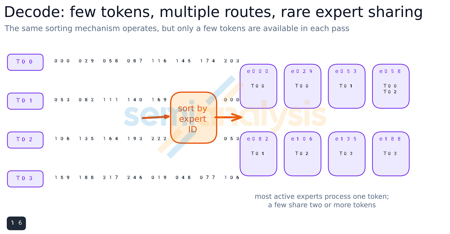
](https://substackcdn.com/image/fetch/$s_!EiMQ!,f_auto,q_auto:good,fl_progressive:steep/https%3A%2F%2Fsubstack-post-media.s3.amazonaws.com%2Fpublic%2Fimages%2Fc0e527fb-7eca-4cd5-9b68-3e8c0c7df672_2312x1203.png)Figure 21. Decode uses multiple routes but rarely shares experts at small batch sizes.

17. Scheduling makes disaggregation useful

Disaggregation becomes most effective as a statistical system at cloud scale. A large pool can contain workers configured for long prefill, short prefill, long-context decode, short-context decode, or other useful classes. The orchestrator assigns each job to a suitable available worker and moves the required KV blobs through shared storage.

Prefill and midfill work are predictable once the prefix size, new-token count, and worker configuration are known. Decode is stochastic because output length is uncertain. Storage between the pools decouples predictable production from irregular consumption. A ready buffer of completed prefill and midfill work can keep decode workers fed even as individual queries finish at different times.

The scheduler should observe customer workloads and time-of-day patterns, anticipate known ramps, and reconfigure workers as the mix changes. Reconfiguration may mean loading different model stages, changing pipeline cardinality, reallocating expert capacity, or moving a rack among prefill, midfill, and decode.

Scale matters. In a small fixed benchmark, one input-fill stage may be connected directly to one decode stage. A slow stage can strand capacity elsewhere in the other stage. In a large pool, workers complete and start independently so no worker need be stranded.

High interactivity and high utilization are therefore not inherently opposed. The scheduler can keep batches small while keeping machines busy, provided it has enough workers, enough storage bandwidth, enough visibility into the work, and fast enough response times to adapt to the moment.

The service overview in Figure 1 provides the corresponding system picture: four resource pools with the orchestrator spanning beneath them.

18. Feedback can turn a small imbalance into oscillation

A tightly coupled system can amplify ordinary variation. Suppose admission to input fill is gated directly by the retirement of decode queries. A long-running decode query delays retirement. Input-fill admission falls. Decode later drains its ready queue and becomes underfed. Admission then opens aggressively, producing a burst of input-fill jobs and a new wave of congestion.

This is a delayed feedback loop. The control signal arrives after the system state has changed. Large batch recovery can make the loop worse by increasing KV-memory pressure and response latency. The factory alternates between full and empty rather than operating near a steady point.

No single scheduler policy solves the problem. Several familiar control techniques help:

use ready-work buffers between stages;

regulate admission from smoothed backlog and predicted service rate rather than individual retirements;

separate fast local controls from slower capacity controls;

apply hysteresis to worker reconfiguration;

reserve capacity for short interactive work;

and avoid changing batch size more quickly than the system can observe its effect.

The same principle extends across timescales. Microsecond worker scheduling, millisecond token flow, second-scale buffers, minute-scale worker reconfiguration, and hour-scale demand planning should not all respond to the same noisy signal.

[
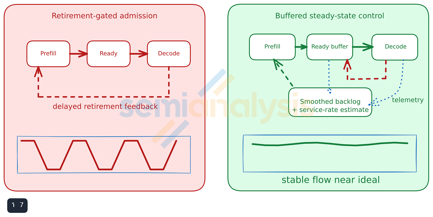
](https://substackcdn.com/image/fetch/$s_!dEj5!,f_auto,q_auto:good,fl_progressive:steep/https%3A%2F%2Fsubstack-post-media.s3.amazonaws.com%2Fpublic%2Fimages%2Fe6442464-d72d-4e1d-a3ff-6d020b0854c5_2090x1046.png)Figure 22. From retirement-gated oscillation to steady flow.

19. Aggregation Compared to Disaggregation

Now that we have exhaustively described disaggregated inference, is there a case to be made for aggregation? To some extent, yes. Clearly, since conversations can pause for minutes and hours it is not reasonable to keep a whole conversation tied to one system. That HBM can be put to better use within seconds of the end of a turn, and modern scaleout networks can move gigabytes of KV cache to a cheaper place in a parallel storage system, which can tier DRAM and SSD, in less than a second.

However, during a turn, do we need to schedule more than one place to get the work done? It is expensive to have too many different designs of server, adding operational costs as well as design work. What if there were only one design, and it centers on the midfill case? A request can be scheduled to that empty worker and stay there for prefill, midfill, and decode. It would need to have enough compute for prefill and midfill, and enough memory bandwidth for decode. There would always be some stranded capacity for either compute or memory transfer, depending on which stage the model is running, but we already tolerate low MFUs on GPUs. We try to overcome that with clever kernels, but in practice clusters run with stranded functions all the time.

Complex orchestration will result in some stranding. Some of that is avoided if a turn runs on a single aggregated worker. No schedule gap when pre/midfill hands over to decode. Natural sharing of one copy of the wide parallel set of experts. No network overhead to move the context from fill to decode. The orchestrator still looks at the shape of the request – cache size, input sequence length, model type, customer interactivity level – and makes one decision which available worker should handle it through all stages of the turn. Then it leaves it alone until the stop token comes out and the turn is delivered to the user and cached to the fast parallel file system. The one worker uses kernels and dataflows adapted to the given request shape as it works through all stages of the turn.

Aggregated workers have their attractions and advocates.

All systems will always strand some capabilities of the accelerators in real world uses. In a disaggregated system there can be two (or more) types of machines built with investment focused on compute, memory, and network actually used, arguably the best use of that investment. Prefill machines might invest in compute, while decode machines might invest in memory. If workers are aggregated, then one machine will be used through all phases so it needs to invest in the strongest compute and the strongest memory thruput. Maybe also strong network. If is not an all-around standout, then it will be held back by its weaker sections and be an overall “meh”. So, aggregation has advantages but it also leaves nowhere to hide in delivering the best of all-around performance. If you can build that magic all around star, then aggregating the whole turn in one worker could be best.

20. Memory bandwidth and memory capacity are different objectives

Memory is often discussed as two independent scalars to maximize. In practice, capacity and bandwidth trade against each other, and their economic value must be considered together.

Data earns revenue when it moves; it incurs cost while sitting idle. An accelerator with very high memory throughput can produce tokens at a rate that lower-bandwidth memory cannot match, even if the lower-bandwidth configuration has more capacity. Capacity is valuable until the active weights, KV state, activations, and operating slack fit cleanly. Beyond that point, additional local capacity may add cost but not revenue.

The capacity curve is not a vertical cliff. Below the useful limit, adding accelerators supplies both more memory and more bandwidth. The advantages end when other limits appear: maximum scale-up width, poor model cuts, the dominance of latencies, extra synchronization, or network contention.

A safe-capacity design point must sit above those limits. It includes margin for realistic context distributions, double buffering, fragmentation, failures, and transient peaks. The revenue-capacity curve rises steeply before that point, rounds smoothly, and then reaches a flatter ceiling determined mainly by bandwidth and compute. Revenue may even decline if excess capacity becomes a sunk cost that operations try to justify with big slow batches of high throughput but inferior value.

Accelerator HBM is too expensive to hold idle data without immediate use. Completed KV blobs should move into CPU DRAM for outgoing staging and then into scale-out storage. Frequently reused common blobs may remain replicated in shared CPU memory or nearby cache appliances. Only the active working set can pay for the most expensive memory.

Tall stacks of high-capacity memory may impose costs in power, signal quality, packaging, and frequency. A design with just enough capacity and exceptional bandwidth may serve interactive inference at higher margins than one that maximizes capacity per accelerator with idle excess.

[
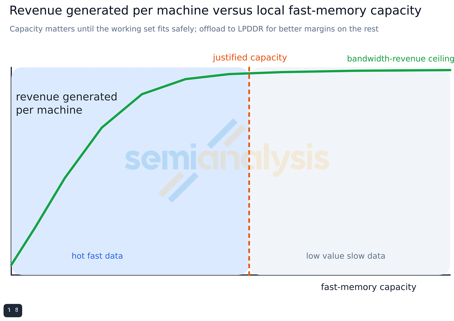
](https://substackcdn.com/image/fetch/$s_!66Yn!,f_auto,q_auto:good,fl_progressive:steep/https%3A%2F%2Fsubstack-post-media.s3.amazonaws.com%2Fpublic%2Fimages%2Fb34940fd-4858-40a2-96c7-8b772840772c_2398x1696.png)Figure 23. Revenue per machine versus local fast-memory capacity.

21. A practical mapping method

The prior sections can be condensed into a repeatable method for mapping a model onto a machine.

Separate the operating regimes. Measure prefill, midfill, decode attention, and decode experts independently. Each may split further by context length or workload class—for example agents, coding, media, or content creation. These become prepared configurations that the orchestrator can mix in production.

Describe the repeating layer group. Identify full and optimized attention, shared transforms, routed experts, and any cross-layer dependency.

Measure active state rather than total parameters alone. Separate stage weights, active experts, live activations, KV state, and transient buffers.

Choose the natural parallel dimension for each operation. Pipeline the layer stack, tensor-parallelize broad indivisible work, and distribute independent experts widely.

Map the broadest operation first. Long-context attention often determines memory striping and the minimum useful scale-up participation.

Place expert weights in regular local destinations. Let routing select among known peer locations rather than creating a global event for every token. A large model may contain on the order of 15,000 layer-experts, and each can be placed with regard to the other experts in its layer and the expected routing distribution. The goal is even use of memory capacity and bandwidth.

Keep repeated high-throughput cooperation inside the strongest fabric. Let thinner activations and amortized KV movement cross weaker boundaries. Respect latency and power cliffs as well as throughput cliffs.

Stop increasing pipeline depth at the KV-memory crossover. Once the model and target context fit with safe margin, additional stages bring little memory benefit and add stage-transition latency.

Use input fill and decode differently. Sort prefill and midfill routes into expert batches; preserve small-batch decode interactivity.

Design storage and scheduling with the worker. KV movement, admission control, ready buffers, and worker reconfiguration determine whether the physical mapping produces steady throughput. Short batches and continuous batch updates let the orchestrator replace individual requests without waiting for the whole batch to retire.

The method does not select one universal topology. It makes the trade-offs visible. A peer set may be one package, one board, or a rack-wide scale-up domain. A layer-group crêpe may map to one node or several. The important point is that the communication hierarchy follows the model’s actual flow.

[
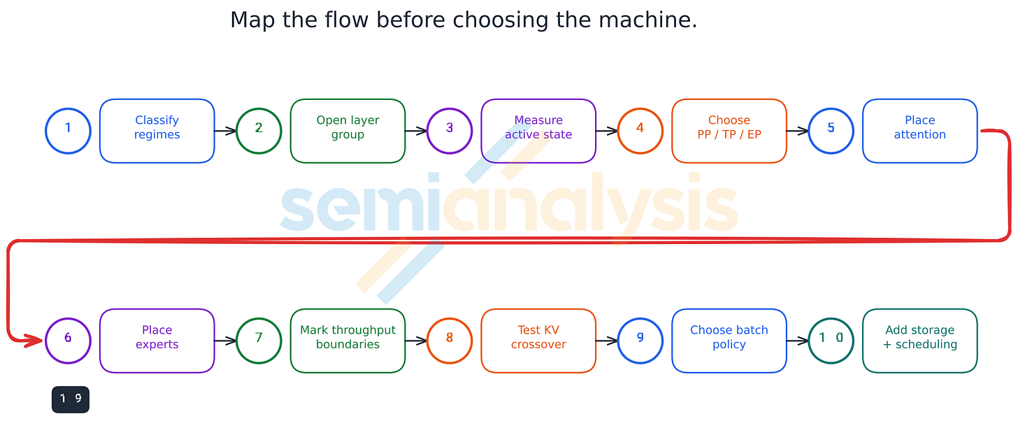
](https://substackcdn.com/image/fetch/$s_!vpdJ!,f_auto,q_auto:good,fl_progressive:steep/https%3A%2F%2Fsubstack-post-media.s3.amazonaws.com%2Fpublic%2Fimages%2F9d85edd1-be4f-481c-a4f9-b48bf9499549_2638x1090.png)Figure 24. A practical sequence for mapping the model onto a worker and then into a token factory.

22. The next view is time

The diagrams so far describe structure and flow. The next step is to place time over them.

Interactive decode has a tight end-to-end budget. Execution of one layer commonly needs to fit within roughly 50 microseconds to 1 millisecond, which across a typical 60-layer model corresponds to roughly 15 to 300 generated tokens per second. Each layer contains several sequential phases, so individual arithmetic operations and handoffs live in tens of microseconds, microseconds, and sometimes fractions of a microsecond.

At that scale, tensor arithmetic is only part of the result. Kernel launch, queueing, synchronization, memory setup, routing, reduction, and link latency must all remain small compared with the operation they support. An expert multiply that takes a fraction of a microsecond is of diluted value if dispatch and data movement take several microseconds each.

The timing view also sharpens the network hierarchy. A high-bandwidth path may still be unsuitable if its setup latency is too large. A small local buffer can be more valuable than a large distant memory tier for a sub-microsecond handoff. A scheduler that creates millisecond variation can overwhelm careful microsecond engineering inside the worker.

The factory spans several control timescales:

local arithmetic and link handoffs in fractions of a microsecond to microseconds;

layer execution in roughly 50 microseconds to 1 millisecond;

token generation in milliseconds;

ready buffers and admission control in roughly 0.1 to 10 seconds;

worker reconfiguration by the orchestrator over seconds to minutes;

KV-blob retention and lifecycle in the fast parallel file system over minutes to days;

and customer demand planning over hours and days.

These loops should be designed separately and joined carefully. Fast controls should not chase slow demand noise, and slow controls should not react to every transient queue fluctuation.

[
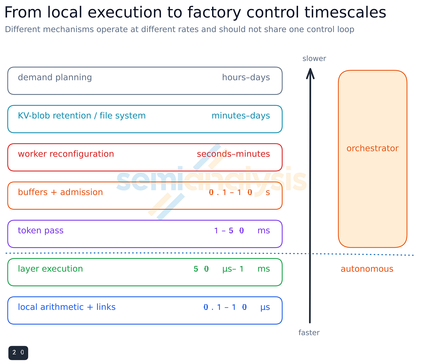
](https://substackcdn.com/image/fetch/$s_!BUH2!,f_auto,q_auto:good,fl_progressive:steep/https%3A%2F%2Fsubstack-post-media.s3.amazonaws.com%2Fpublic%2Fimages%2Ff1ddae71-31af-4a95-8b42-61c3f24bfd5a_2096x1807.png)Figure 25. From local execution to factory-control timescales.

23. Worked example: projected Kimi K3 performance on Blackwell systems

The preceding sections describe a method for reasoning about model placement. A useful check is to apply it to a specific frontier model and explore the resulting trade-offs together. The following charts show modeled Kimi K3 performance on B200, B300, and GB200 systems using configurations from 16 to 64 GPUs in a rack. These are workload-and-hardware projections, not measured benchmark results. Connected lines identify projected Pareto frontiers: configurations for which interactivity cannot improve without giving up throughput or another selected objective.

22.1 Interactivity and throughput

The first chart compares time per output token for decode, or time to first token for prefill and midfill, against tokens per second per GPU. Normalizing throughput per GPU makes configurations of different sizes directly comparable.

The lower-left group contains decode frontiers for 8k and 32k input contexts. Feasible configurations appear for all three GPU types. GB200 is strong across much of the frontier, while B200 and B300 also offer competitive points. The lowest-latency decode configurations generally combine pipeline and tensor parallelism. At the throughput-oriented end, the highest tokens per second per GPU tend to come from one attention instance per GPU, without tensor or pipeline parallelism, while expert parallelism remains as wide as the system permits.

The upper-middle group is midfill: 127k cached input tokens followed by a 1k-token append before decode. GB200 leads the low-TTFT portion without pipeline parallelism, using TP=4 or TP=2. B300 catches up toward the throughput-oriented end. B200 and B300 generally use PP=4, with expert parallelism bounded within each stage so the expert all-to-all remains inside the node.

The two groups at upper right are 8k- and 32k-token prefills. All three GPU types converge on similar configurations: PP=4, with TP=4 or TP=2 favoring lower TTFT at some cost in throughput. Their close projected performance reflects the shared Blackwell compute architecture and the compute-limited nature of these prefill workloads.

[
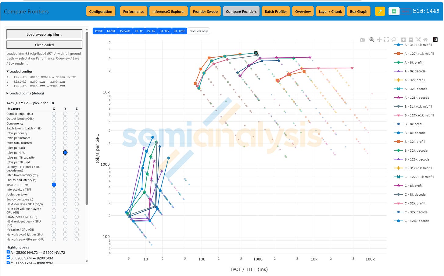
](https://substackcdn.com/image/fetch/$s_!4rOA!,f_auto,q_auto:good,fl_progressive:steep/https%3A%2F%2Fsubstack-post-media.s3.amazonaws.com%2Fpublic%2Fimages%2F3f424d0d-368f-461d-8b78-5433bed03128_2048x1274.png)Figure 26. Projected interactivity and throughput frontiers for decode, midfill, and prefill. Source: SemiAnalysis Inference Simulator.

22.2 Energy per query

The second chart uses the same simulated configurations but changes the vertical axis to energy per completed query. Decode is the largest energy workload because the modeled output length is 1,000 tokens, requiring roughly 1,000 passes through the model for every query. Midfill uses the least energy: it appends a relatively short sequence after one pass through an existing long context. Full 8k and 32k prefills require successively more energy.

The model includes Kimi K3’s localized-attention layers, so both retained state and computation reflect the expected savings from the attention structure rather than treating every layer as full attention.

[
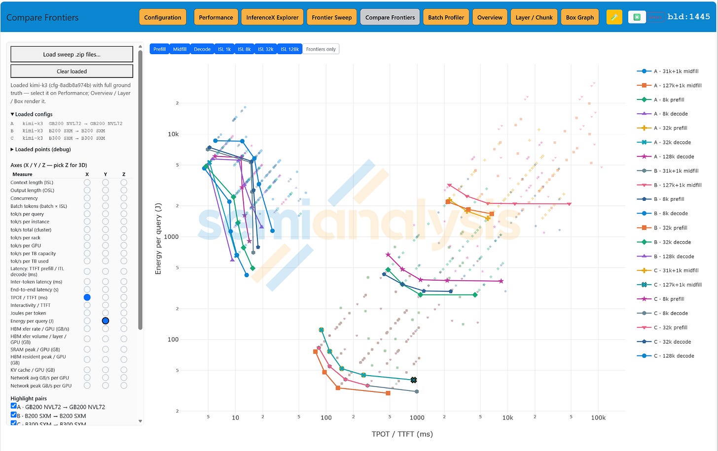
](https://substackcdn.com/image/fetch/$s_!L_rU!,f_auto,q_auto:good,fl_progressive:steep/https%3A%2F%2Fsubstack-post-media.s3.amazonaws.com%2Fpublic%2Fimages%2F0ab3a5dc-803c-4d91-b513-ca10e9ea2df6_2048x1289.png)Figure 27. Projected energy per query for the same decode, midfill, and prefill frontiers. Source: SemiAnalysis Inference Simulator.

22.3 Fast-memory requirements

The third chart shows peak HBM residency per GPU. It excludes the extra buffers used while KV state enters or leaves the worker, which may add several gigabytes per GPU. Between conversational or agentic turns, inactive KV blobs can be transferred in parallel to network-attached DDR, including the DRAM attached to node CPUs. That memory is cheaper, more available, and less constrained by the HBM supply chain.

The projected frontiers cluster near the lower end of the feasible memory range. For prefill and midfill, the downward steps come from adding pipeline parallelism and increasing tensor or data parallelism, including data-parallel ring-batched instances. Decode reduces per-GPU residency first through tensor or data parallelism, using pipeline parallelism later.

Most frontier configurations remain below approximately 80 GB per GPU even after allowing for practical KV-transfer buffers. This supports the earlier conclusion that bandwidth can be more valuable than maximizing HBM capacity on every accelerator, provided the broader storage and orchestration system moves idle state promptly.

[
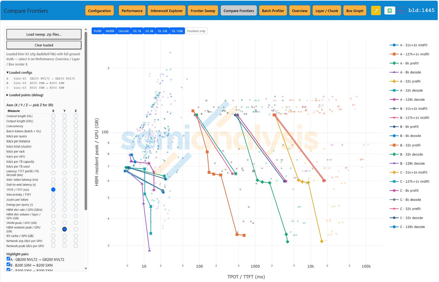
](https://substackcdn.com/image/fetch/$s_!-v6T!,f_auto,q_auto:good,fl_progressive:steep/https%3A%2F%2Fsubstack-post-media.s3.amazonaws.com%2Fpublic%2Fimages%2Faf12d141-27cf-4c91-9532-9978c5a3a792_2792x1796.png)Figure 28. Projected peak HBM residency per GPU across the simulated frontiers. Source: SemiAnalysis Inference Simulator.

22.4 Network peaks and the scale-up boundary

The fourth chart shows projected peak network traffic per GPU. Prefill and midfill make intensive use of the network for expert parallelism because many routed activations are in flight at once. Pipeline parallelism is therefore particularly useful on B200 and B300 systems: placing one stage inside a node keeps its expert all-to-all traffic on the local NVLink fabric.

GB200 NVL72 extends scale-up bandwidth across the rack. More GPUs can therefore participate in one layer in parallel, with all instances advancing through that layer in synchrony, to improve latency and throughput without crossing a weaker network boundary.

Decode shows lower interval-averaged peaks because a small batch consults relatively few experts at once. Individual transfers still burst at the physical NVLink rate; the lower plotted value reflects a measurement interval longer than the transfers themselves. This distinction between instantaneous link rate and sustained traffic matters when sizing the fabric and interpreting utilization.

[
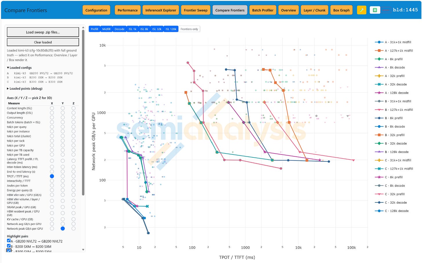
](https://substackcdn.com/image/fetch/$s_!485f!,f_auto,q_auto:good,fl_progressive:steep/https%3A%2F%2Fsubstack-post-media.s3.amazonaws.com%2Fpublic%2Fimages%2F8f02faa0-a5dd-4f3f-bc27-37c4f6912894_2652x1652.png)Figure 29. Projected peak network traffic per GPU and the benefit of keeping expert traffic inside the scale-up domain. Source: SemiAnalysis Inference Simulator.

The four views tell a consistent story. The best configuration changes with the operating regime and the selected point on the latency-throughput frontier. Prefill and midfill reward organized parallelism and stage-local expert traffic. Decode benefits from parallelism at the low-latency end, but the highest throughput per GPU comes from simpler attention instances combined with wide expert placement. Across the projected frontiers, fast-memory capacity appears less restrictive than network placement, memory bandwidth, and orchestration.

Closing perspective

The useful unit of analysis for inference is not total parameter count alone. It is the active flow of the model joined to the memory, communication, and timing hierarchy of the machine.

MoE provides structure. Layer groups repeat. Experts are numerous but individually manageable. Attention is broad and increasingly shaped by KV state. Operations occur in sequence and can reuse hardware. Pipeline, tensor, and expert parallelism can each follow the dimension where it is most natural. Prefill and midfill can sort routes into efficient expert batches, while decode can preserve short batches and high interactivity.

The hardware can reflect that structure. A logical accelerator peer set provides a bounded scale-up domain. Nodes stack into racks. A rack may be one scale-up worker or several pipeline stages. Shared storage makes KV blobs movable. Datacenter networking connects bounded workers rather than carrying every inner tensor operation. Scheduling keeps predictable and stochastic stages in steady flow.

Holding the problem this way does not remove its scale. It makes that scale easier to divide. The model, worker, rack, storage system, and scheduler become parts of one coherent design that can be measured, illustrated, and improved.

📋 讨论归档

讨论进行中…