在阅读本文的过程中,你将从零开始建立数据科学技术、风险与收益建模、数据可视化等方面的基础。
无论你是第一次在编程语言里接触金融概念,还是只是想温习基础知识,你都来对地方了。
这里的每个概念都配有可运行的 Python 代码,而且每一节都在上一节的基础上继续推进,所以不要跳着读。
免责声明:非投资建议 & 请自行研究 & 市场有风险
让我们开始吧!
数据来源:
1 - NumPy Python 中使用最广泛的数值计算库,用于处理数组、矩阵和数学运算:
max_dd_date = drawdowns.idxmin()
print(f"Date: {max_dd_date}")
2 - Pandas 一个 NumPy 的封装库,我们将用它把数据放在带标签的结构中,让金融分析真正变得可控:
vol = returns.std()
print(vol)
3 - Matplotlib 我们的数据可视化工具,把数字变成图表:
4 - Read_csv 要把数据导入 pandas,我们可以使用 read_csv 函数,并传入本地文件路径或远程托管资源的 URL:
5 - Yfinance 我们将不再使用 CSV 文件,而是使用一个名为 yfinance 的 Python 库来抓取数据,它会把数据放进 pandas 的数据结构里:
type(prices) # pandas.core.frame.DataFrame
6 - Yf . download 我们来下载 ETF:SPY 的月度股价:
returns = prices.pct_change()
7 - Adjusted Close Adjusted Close(复权收盘价)给我们的收盘价会把分红、拆股等现金流因素计入其中,这样我们就不会漏掉任何数据。用它计算得到的是总回报(total returns),而不是仅价格回报(price returns):
display = (total_return * 100).round(2).astype(str) + "%"
print(display)
一只股票每年派息 3%,在原始 Close(收盘价)图上可能看起来是横盘,但你其实是赚了钱的。20 年下来,这个差距会复利到 80% 以上。
一定要使用 Adjusted Close。
信息准备
8 - Series pandas 有两种不同的数据结构可以用来存储数据。Series 是一维的,可用于单只股票的数据:
import yfinance as yf
9 - DataFrame DataFrame 是二维的,可用于存储多只股票的数据:
start = returns.index.min() - pd.DateOffset(months=1)
在本文中我们将始终使用 DataFrame。
10 - Dropna and inplace 当两只股票的起始日期不同导致出现 NA 值时,我们可以调用 dropna 来删除所有包含 NA 的行。
inplace 参数会在现有 DataFrame 上直接执行操作,而不是返回一个新的对象:
r1, r2, r3 = 0.10, -0.05, 0.08

compound = (1 + r1) * (1 + r2) * (1 + r3) - 1
print(f"Compound: {compound:.4%}")  # 13.34%
11 - Price Series 我们现在拥有的是所谓的价格序列(price series),因为我们在连续的时间步上都有价格数据。
12 - Index 日期列很特殊,它被称为我们的索引(index)。
我们可以用 to_period 方法把索引的格式改为按月,以匹配数据的粒度:
prices.plot()
plt.title("Price Series")
plt.show()
13 - Plotting Prices 现在我们可以用 matplotlib 来绘制价格:
prices.dropna(inplace=True)
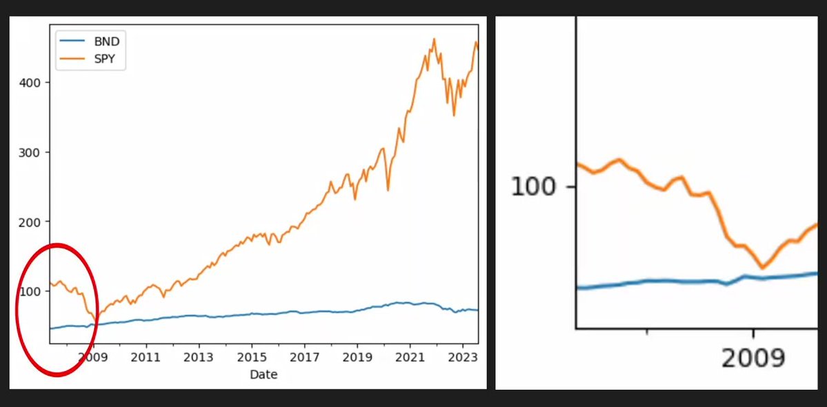
但这其实并不能帮助我们进行任何比较,因为当前这些价格只是原始的 ETF 数据,它们从两个不同的任意起点开始。
我们很快会用财富指数(wealth index)来纠正这一点。
max_dd = drawdowns.min()
print(f"Max Drawdown: {max_dd}")
收益率
在从价格计算收益率之前,我们先回顾一些基础数学。
14 - Standart Return Formula 你很可能学过最常见的收益率公式:用资产最终价格减去初始价格,再除以初始价格:
Return = (P_final - P_initial) / P_initial
这会给出一个单期收益率(用小数表示),然后你可以把它转换成百分比:
prices.iloc[0]
prices.iloc[0:12]
15 - 1+R Format 稍微改一下标准公式会很有帮助。如果我们用最终价格除以初始价格,我们得到的数字与原本等价,但会大 1。
然后再减去 1,就回到完全相同的结果:
total_return = (1 + returns).prod() - 1
这称为 1+R 格式(1+R format),它会在全文反复出现。
16 - Multi-Period Return 以上都只是单期收益率。
要计算多期收益率,我们可以对每个单期收益率都加 1,把它们全部相乘,然后再减 1:
Compound Return = (1+r₁) x (1+r₂) x ... x (1+rₙ) - 1
prices.size
这称为复利收益(compound)或几何收益(geometric return)。这个过程叫做几何链接(geometric linking)。
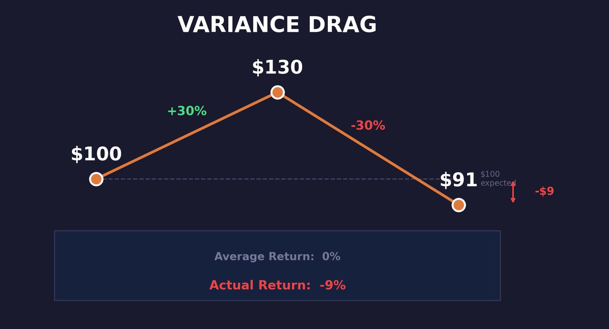
17 - Variance Drag 需要注意的是:要计算复利收益(也就是实际收益),你不能简单把收益率加总,因为存在所谓的“方差拖累”(variance drag)。
如果你向某资产投入 $100,在第一个时间步赚了 30%,那就是 $100 的 30%。
如果在第二个时间步亏了 30%,那就是 $130 的 30%,也就是 $39:
import numpy as np
import pandas as pd
import matplotlib.pyplot as plt
import yfinance as yf

# Data
prices = yf.download(["SPY", "AGG"], period="max", interval="1mo")["Adj Close"]
prices.dropna(inplace=True)
prices.index = prices.index.to_period("M")

# Returns
returns = prices.pct_change().dropna()

# Metrics
total_return = (1 + returns).prod() - 1
ann_ret = lambda r: ((1+r).prod()) ** (12/r.shape[0]) - 1
ann_vol = lambda r: r.std() * np.sqrt(12)
sharpe = ann_ret(returns) / ann_vol(returns)

# Wealth & Drawdowns
wealth = (1 + returns).cumprod()
peaks = wealth.cummax()
dd = (wealth - peaks) / peaks

print("Compound Returns:")
print((total_return * 100).round(2).astype(str) + "%")
print(f"\nAnnualized Return:\n{(ann_ret(returns)*100).round(2)}%")
print(f"\nAnnualized Vol:\n{(ann_vol(returns)*100).round(2)}%")
print(f"\nSharpe:\n{sharpe.round(3)}")
print(f"\nMax Drawdown:\n{(dd.min()*100).round(2)}%")
def annualize_vol(returns, periods_per_year):
    return returns.std() * np.sqrt(periods_per_year)

ann_vol = annualize_vol(returns, 12)
print(ann_vol)
平均收益率是 0%。实际收益率是 -9%
算术收益与几何收益之间的差距大约是 σ²/2 ,并且会随着波动率的平方增长。
年化波动率 20% 时,拖累约为 ~2%/年
波动率 80% 时则约为 ~32%
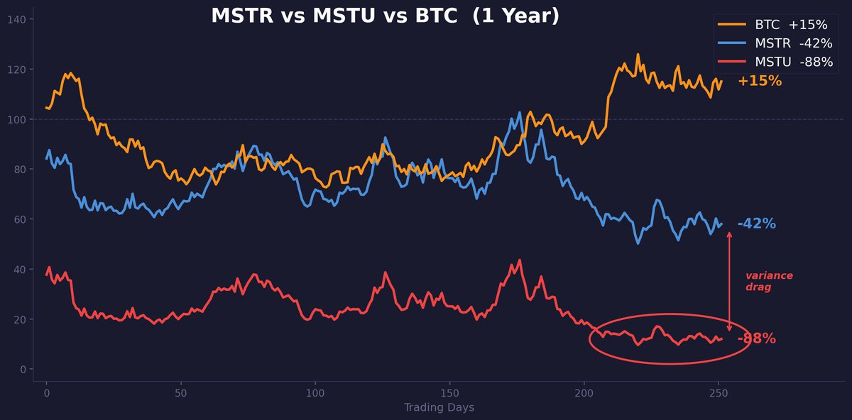
如果你觉得这只是理论,看看 MSTU——2 倍杠杆的 MicroStrategy ETF。
过去一年里,MSTR 大约下跌了 42%,而 btc 实际上涨了 15%。MSTU 并没有下跌 84%,而是下跌了 88%。
这些额外的损失纯粹是方差拖累:在一只已实现波动率 90%+ 的标的上,它每天都在对持有人进行复利式的反向侵蚀。
同一年里,2 倍做多和 2 倍反向的 MSTR ETF 都跌去了 65% 以上。无论做多还是做空,双双被摧毁。
这就是方差拖累在现实世界中的运作方式。
p_initial = 100
p_final = 130

ret = (p_final - p_initial) / p_initial
print(f"{ret:.2%}")  # 30.00%
如果你只从本文学到一件事,那就学这件事。
18 - Pct_change 如果你想把价格序列转换为收益率序列,可以走捷径:直接调用 pct_change 方法,而不必使用上面的公式:
drawdowns.plot(title="Drawdowns")

plt.annotate(
    f"Max DD: {max_dd.min():.2%}",
    xy=(max_dd_date.values[0], max_dd.min()),
    xytext=(max_dd_date.values[0], max_dd.min() + 0.05),
    arrowprops=dict(arrowstyle="->"),
    fontsize=9
)
plt.show()
19 - First Data Point Loss 从价格转换为收益率时,你总会丢失一个数据点,因为第一天缺少前一日收盘价,无法计算收益率。
我们可以用 dropna 来清理:
prices.head()
prices.head(10)
现在我们有了收益率序列。
20 - Plotting Returns 如果你想看看收益率长什么样,我们也可以再次绘图:
def annualize_return(returns, periods_per_year):
    compound_growth = (1 + returns).prod()
    n_periods = returns.shape[0]
    return compound_growth ** (periods_per_year / n_periods) - 1
21 - Compounding the Series (.prod) 如果我们想对整个收益率序列进行复利计算,可以先对每个单期收益率加 1,然后调用 .prod() 来计算它们的连乘,最后再减 1:
initial = 100
after_gain = initial * 1.30   # $130
after_loss = after_gain * 0.70  # $91

print(f"Start:    ${initial}")
print(f"+30%:     ${after_gain}")
print(f"-30%:     ${after_loss}")
print(f"Average:   0%")
print(f"Actual:   {(after_loss/initial - 1):.0%}")  # -9%
22 - Formatting Output 如果你想更清晰地查看结果,我们可以先 round,再用 .astype 把数值转换成字符串:
prices = yf.download("SPY", period="max", interval="1mo")
这些就是我们样本内的复利收益。
DataFrame 方法
回到一些 DataFrame 的常用方法。
23 - Head() 查看前五条或前 n 条:
prices.index = prices.index.to_period("M")
24 - Tail() 同理,查看末尾:
arrowprops=dict(
    arrowstyle="->",
    color="red",
    lw=1.5
)
25 - Size 查看 DataFrame 的元素总数:
returns.plot()
plt.title("Return Series")
plt.show()
26 - Shape 查看每个轴的大小:
drawdowns = (wealth_index - previous_peaks) / previous_peaks
27 - Index 查看日期:
prices.loc["2025-01"]
prices.loc["2025-01":"2026-06"]  # slicing with colon
28 - Columns 查看股票:
fig, axes = plt.subplots(2, 2, figsize=(14, 10))

prices.plot(ax=axes[0, 0], title="Prices")
returns.plot(ax=axes[0, 1], title="Returns")
wealth_index.plot(ax=axes[1, 0], title="Wealth Index")
drawdowns.plot(ax=axes[1, 1], title="Drawdowns")

plt.tight_layout()
plt.show()
29 - Single Bracket Indexing 我们可以用单中括号索引单只股票,并得到一个 Series:
prices = yf.download(
    ["SPY", "AGG"],
    period="max",
    interval="1mo"
)["Adj Close"]
30 - Double Bracket Indexing 也可以用双中括号选择任意数量的股票,并保持 DataFrame 的结构:
ann_ret = annualize_return(returns, 12)  # 12 for monthly data
print(ann_ret)
31 - Loc 我们可以通过索引标签,用 .loc 跨行索引:
import pandas as pd
32 - Iloc 或者用 .iloc,通过索引的位置(整数位置)来索引:
wealth_index = (1 + returns).cumprod()
wealth_index.plot(title="Growth of $1")
plt.show()
这两种方法也都支持用冒号运算符进行切片,从而选择一个范围。
风险度量
33 - Standard Deviation 我们来计算以标准差衡量的波动率。
我们知道,标准差就是方差的平方根:
σ = √Variance
同样,我们可以用 .std() 方法来简写底层数学运算:
现在我们已经知道如何计算收益率和波动率,接下来把这两个指标都年化——这才是我们实际用来分析绩效的方式。
年化
34 - Annualized Return 我们知道,如果只有一个月度收益率,可以把它的 (1+r) 提到 12 次方,从而得到等价的 12 个月复利收益。
但现实中我们有一个包含数百个不同单期收益率的序列。我们可以反推:把复合增长(compound growth)提到(每年期数 / 总期数)的幂:
prices.tail()
prices.tail(3)
这里也可以做简写:把复合增长提到(每年期数 / 总期数)的幂。
我们把它写成一个函数,让 periods_per_year 变成可参数化的输入:
one_plus_r = p_final / p_initial  # 1.30
ret = one_plus_r - 1              # 0.30
35 - Annualized Volatility 年化波动率会简单得多:我们只需要把波动率乘以“每年期数”的平方根。
为什么是平方根?因为方差随时间线性缩放。
标准差是方差的平方根,因此 std 随 √time 缩放。
原始夏普比率
36 - Raw Sharpe Ratio 顺便,我们可以计算原始夏普比率(raw Sharpe ratio),它本质上是一个风险调整后的收益指标。
要计算原始夏普比率,我们可以用年化收益除以年化波动率:
subset = prices[["SPY", "AGG"]]
夏普低于 0.5 很弱;0.5 到 1.0 是股票的平均水平;高于 1.0 很强;高于 2.0 则是另一个层级。
有件事大多数人不知道:比特币在 2025 年的 12 个月夏普比率曾达到 2.4,这让它按风险调整收益算进入了全球资产前 100。
那些喊着 “这就是赌博” 的人,从来没有算过这个。
37 - Risk-Free Rate 要计算真正的夏普比率,需要一条国库券(T-bill)收益率的时间序列,也就是无风险利率:
**Sharpe = (R_portfolio - R_f) / σ_portfolio
**这部分会单独讲。做快速对比时,原始夏普已经能帮你走完大部分路。
财富指数
38 - Wealth Index (.cumprod) 如果我们想用收益率序列创建财富指数,可以先对所有收益率加 1,但不再调用 .prod(),而是调用 .cumprod()。它会计算累计乘积,也就是在每个连续时间戳上的“运行乘积”(running product):
previous_peaks = wealth_index.cummax()
现在我们可以对证券进行准确比较。这也代表了一美元的增长路径。
39 - DateOffset 需要注意的是:财富指数其实不是从 1 开始的,因为第一个数据点代表的是第一天的收益率。
如果你想在财富指数中把第一个数据点设为一个静态的 1,可以用 .index.min() 取开始日期,再用 pd.DateOffset 回退到上一个月:
import numpy as np
40 - Pd.concat 然后用 pd.concat 把它前置拼接进 DataFrame:
returns.dropna(inplace=True)
现在每个资产都从 $1 开始,你比较的是实际表现,而不是任意的价格水平。
回撤
最后一个主题:计算并绘制回撤。回撤就是从前一高点到当前价格的收益率变化。
41 - Previous Peaks (.cummax) 我们将用财富指数来帮助计算回撤,并结合前一高点。前一高点可以通过对财富指数调用 .cummax() 得到:
prices.shape # (rows, columns)
cummax 是累计最大值:在每个时间步,它会把数值设为该时间步及之前的最高数据点。
42 - Drawdown Formula 要得到回撤,我们取财富指数与前一高点之差,再除以前一高点进行缩放:
import matplotlib.pyplot as plt
这就是我们的回撤序列。
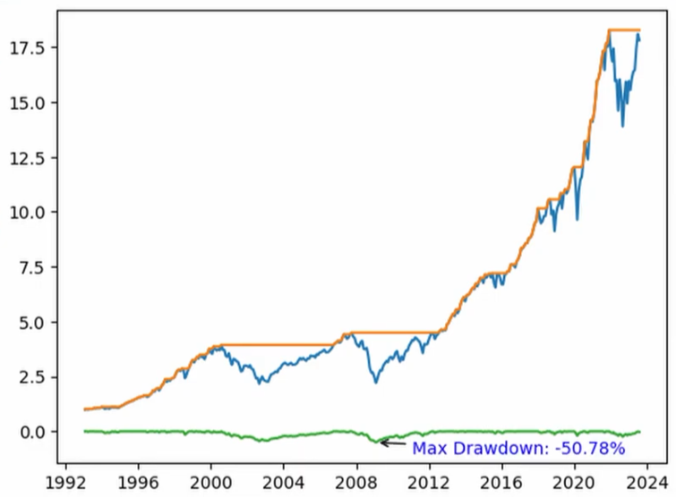
43 - Maximum Drawdown 一个经常计算的关键统计量是最大回撤(maximum drawdown)。因为回撤是负数,我们可以用 .min() 来得到它:
sharpe = annualize_return(returns, 12) / annualize_vol(returns, 12)
print(f"Raw Sharpe: {sharpe}")
44 - Date of Maximum Drawdown 我们可以调用 .idxmin(),也就是 “index minimum”,来得到最大回撤对应的日期:
45 - Matplotlib Annotation 如果你想把这些一起画出来,我们可以添加 matplotlib 标注(annotation):格式化最大回撤,给出坐标、位置,并添加箭头:
spy = prices["SPY"]
这样就把那些可能很难理解的代码,变成清晰的可视化图表。
spy = prices["SPY"]
type(spy)  # pandas.core.series.Series
46 - Arrow Formatting arrowprops 字典控制标注箭头的样式。
你可以自定义样式、颜色和宽度:
prices.columns
47 - Subplots 把所有图放在同一屏幕上查看:
base = pd.DataFrame(
    {col: [1.0] for col in returns.columns},
    index=[start]
)
wealth_index = pd.concat([base, wealth_index])
wealth_index.plot(title="Wealth Index")
plt.show()
同一份数据的四种视图。这是你在任何量化交易员屏幕上都会看到的标准布局。
**48 - Why Drawdowns > Volatility
**波动率把收益和亏损一视同仁:+5% 的一天和 -5% 的一天,对标准差的贡献完全一样。
回撤只衡量下行——也就是你在账户里真正“感受到”的那部分。
一个策略年化 15%、最大回撤 -20%,与另一个年化 15%、最大回撤 -60% 的策略,可能会显示出相似的夏普。
但持有它们时,你的睡眠质量会截然不同。
49 - The Full Pipeline !完整的分析流程:从头到尾,一段可运行的代码块:
df = pd.read_csv("path/to/data.csv")
# or from a URL:
df = pd.read_csv("https://example.com/prices.csv")
复制这段代码,运行它,把 ticker 换成你持有的任何标的。
**50 - What Comes Next
**量化金融里更高级的一切——从期权定价与 Black-Scholes,到蒙特卡洛模拟与因子回归——都是直接建立在这 50 个概念之上的。